Home | Show all

Tutorial


Persistence diagrams and filaments

In this tutorial, we will identify the persistent filamentary structures in a diHydrogen column density map of the interstellar medium in the Eagle Nebula (M16) as observed by Herschel . The map is encoded in a 2D double precision FITS image, with pixels set to NaN in unobserved regions:

M16_blue.png

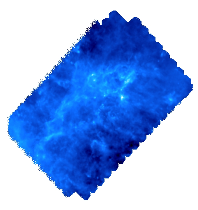
By default, mse will automatically mask NaN valued pixels so the FITS file could theoretically be fed directly to it. However, because of the complexity of the geometry of the observed region, it is preferable to use a mask to limit the analysis to a well defined region of interest (in particular, it is preferable that this region is simply connected - i.e. does not contain holes -). Designing a mask is relatively simple, as it consists in an image with pixels set to 0 in non-masked region and any other value in the masked regions (this behavior can be changed by adding a trailing '~' to the mask filename, see option -mask). The following mask was created with Gimp and saved as a .PNG file (any readable field file format is acceptable):

M16_mask.png


With this mask, we can now use mse to identify the filamentary structures in the map (option -upSkl) with the help of an interactive persitence diagram (option -interactive) to select the correct persistent threshold as we do not want to impose any à-priori on its value. We therefore run the following command:

mse m16_zo_no70um_density.fits -mask M16_mask.png -interactive -upSkl


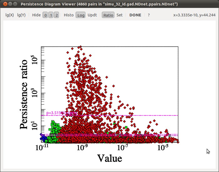
After some computations, the following diagram should appear (use buttons logX/logY to switch logarithmic coordinate and buttons 1, 2 and 3 to show/hide different types of persistence pairs):

M16_persistence_diagram_2.png

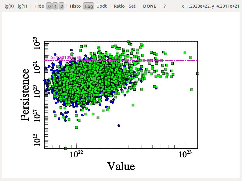
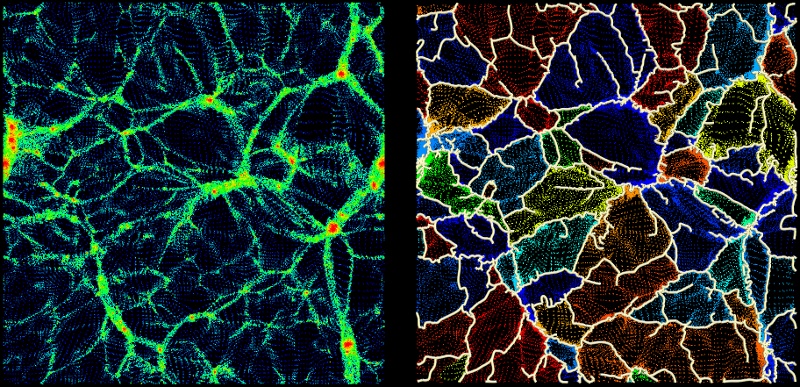
On this diagram, each dot represents a persistence pair of critical points (see overview section), with its X coordinate being the value at the lowest critical point of the two (i.e. the background density) and its Y coordinate the persitence of the pair (i.e. the value difference between the two, interpreted as contrast of the topological feature it represents with respect to its background). Points located in the right side of this diagram represent features located in high valued regions of the map, while points in the upper side represent features that clearly stand out from their background. More specifically, the green squares stand for pairs of type 1 (i.e. saddle-point / maximum pairs) while blue disks stand for pairs of type 0 (i.e. minimum saddle-point pairs). This can be easily visualized on the following image, which represents a zoom on the map with critical points identified as blue squares, green crosses and red triangles for minima, saddle points and maxima respectively. On this plot, the identified filaments are represented in black, and each persistence pair of type 0 or 1 is represented as a blue or green segment linking its two critical points together (each segment corresponds to one point in the persistence diagram above):

M16_skel_nocut_ppairs_crit.png

Basically, in 2D, removing a pair of type 0 (i.e. cancelling two critical points linked by a blue segment) amounts to deleting a piece of filament (i.e. 2 arcs departing from the saddle point) by merging two voids while removing a pair of type 1 (i.e. cancelling two critical points linked by a green segment) amounts to gluing pieces of filaments into longer ones (i.e. two arcs departing from the saddle point with one other arc departing from the maximum). When selecting the persistence threshold without à-priori, we therefore want to keep only the pairs that stand out of the general distribution on the Y-axis (i.e. with high persitence) so that only the most significant topological features remain. Selecting a threshold of ~4.2E21 as shown on the persistence diagram above seems quite reasonable (using Ctrl+left Click, and clicking on the DONE button to proceed).

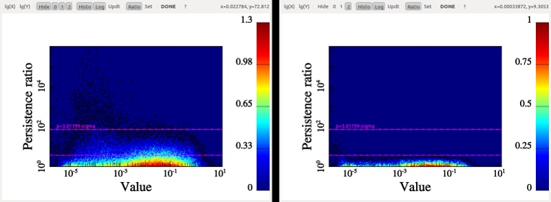
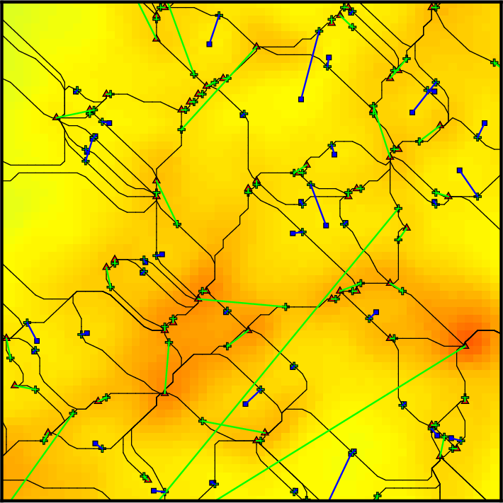
Visualizing a persistence diagram is a good way to determine the persistence threshold when assuming no previous knowledge of the data set. Note however that persistence could also have been set à-priori to the estimated amplitude of what is considered non-meaningful features or noise with option -cut <val> instead of -interactive. It is nonetheless always useful to check the persistence diagram as it deeply reflects the topological nature of the distribution and can be used to understand it better. For instance, the following diagram (represented by a 2D histogram of the pairs distribution, instead of the pairs themselves) was computed from a totally different map, and it is a good example:

ic5146_col_dens_pers_diag.png

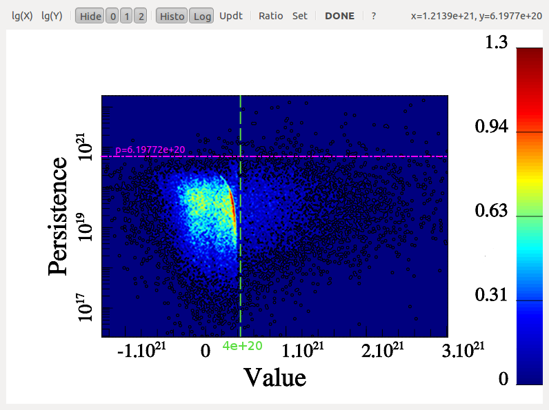
Indeed, from this diagram, not only can one learn that the persistence threshold should be ~6.E20 (from the Y-axis), but one can easily see that the nature of the distribution is different for background values below or above "X=~4E20" on the X-axis. This feature reflects the fact that in some regions of this data-set, the signal was below the instrument detection threshold and the result is complex noise generated by the detectors. Meaningful features may stand out from these regions, so it does not affect the choice of the persistence threshold. However, this tells us that any region with a value <4E20 cannot be considered signal and identified filaments should therefore be trimmed wherever the value is below this threshold (this can be achieved by running mse with a persitencce threhold of 6.E20 and then running the following command on the output skeleton file: skelconv filaments.NDskl -trimBelow 4.E20).

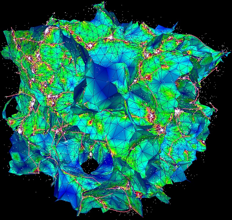
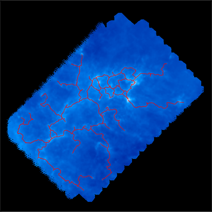
Let us now come back to our example, where no such trimming is necessary. Selecting a persistence threshold of ~4.2E21 as discussed previously, we obtain the following filamentary structures :

M16_skel.png

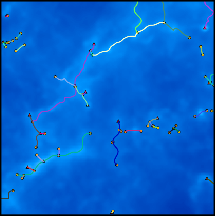
Remember that DisPerSE identifies structures as features of the Morse-Smale complex. The output of mse is always a valid (subset of the) Morse-Smale complex. In particular, filaments are identified as the set of arcs joining maxima and critical points, which means that pieces of filament always link a maximum and a critical point: they cannot stop in any other point, and whenever two filaments merge in points that are not maxima (i.e. bifurcation point), they remain distinct filaments until they reach a maximum (i.e. although they are not visually distinct as they are infinitely close, they are still stored as separate arcs in the output file). This is illustrated on the following figure, which shows a zoom on the identified filamentary structures with minima, saddle points and maxima represented as blue squares, green crosses and red triangles respectively:

M16_skel_nodes.png

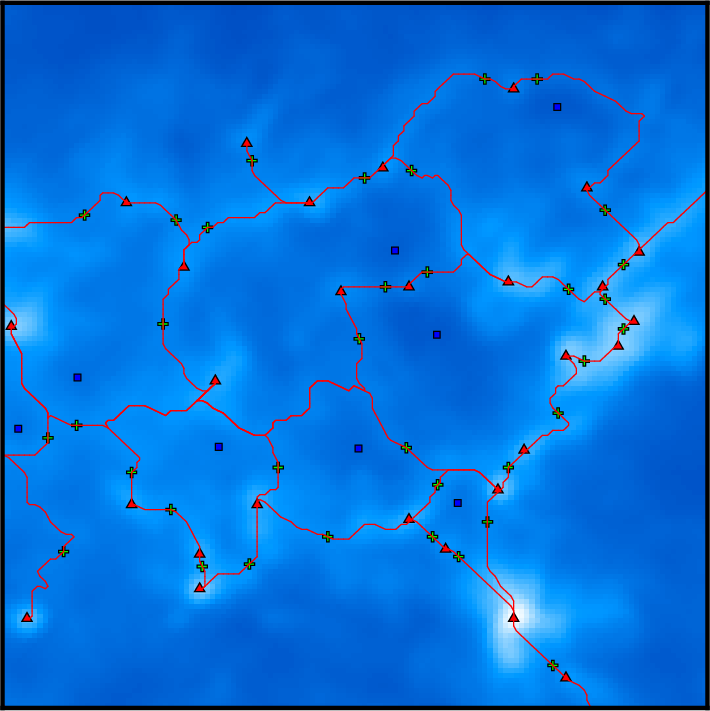
On this figure, individual pieces of filaments (i.e. arcs) link red triangles to green crosses, and several pieces of arcs may therefore overlap above bifurcation points. This is of course desirable for mathematical applications that require the computation of valid Morse-Smale complexes but can be problematic when one only needs to identify structures and measure their properties. Indeed, regions where several arcs overlap may accidentally be given a stronger weight in statistical analysis, biasing the results. One can fix this with the option -breakdown of skelconv which is used to identify bifurcation points (adding them as dummy critical points of critical index D+1) and break filaments down into individual pieces of arcs.

Another problem is the resolution of the filaments, which is roughly equal to that of the underlying map: filaments are described as sets of small segments linking neighbor pixels together in the oupout files of mse. As a result, they appear jagged on the previous image and they can locally only take a discrete set of orientation. Using option -smooth N of skelconv, one can fix this by ensuring their smoothness over a size of ~N pixels. Note that only individual arcs or pieces of arcs are smoothed when using this option, critical points and bifurcation points remain fixed. As a result, the order of options -smooth and -breakdown on the command line is important.
We choose to first smooth over ~6 pixels and then break the network down :

skelconv m16_zo_no70um_density.fits_c4.2e+21.up.NDskl -smooth 6 -breakdown


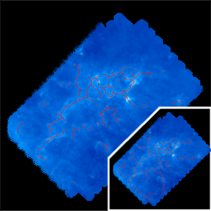
The result is illustrated on the following figure:

M16_skelBS_nodes.png

where filaments are now smooth and bifurcation points are now identified as yellow discs : pieces of filament now link critical or bifurcation points and therefore do not overlap anymore.

Although the resulting filaments are perfectly usable as such for analysis, other useful post-treatment are available in DisPerSE. We give in the following an example of their possible usage, but note that it should of course be adapted to the particular results one wants to obtain ...

Options -trimAbove and -trimBelow for instance allow trimming portion of arcs so that they do not have to start/stop at critical or bifurcation points (dummy critical nodes are added at their extremities). By default, these options will trim the filaments above or below a given value of the field (see e.g. the example in the section on the persistence diagram above), but filaments can also be trimmed in any value tagged within the skeleton file (the list of the tags can be displayed by running skelconv filaments.NDskl -info and arbitrary tags can be added with option -addField).

A useful trimming function is robustness or robustness_ratio, which is not tagged by default in the skeleton files but can computed using option -robustness of mse (you can use option -loadMSC to avoid recomputing the whole Morse-Smale complex):

mse m16_zo_no70um_density.fits -mask M16_mask.png -cut 4.2E21 -upSkl -loadMSC m16_zo_no70um_density.fits.MSC


Robustness implements an improved version of the concept of separatrix persistence (Weinkauf, T. and Gunther, D., 2009) that allows the extension of regular persistence to each points of the filaments (as opposed to critical points pairs). Running the following command:

skelconv m16_zo_no70um_density.fits_c4.2e+21.up.NDskl -breakdown -smooth 6 -trimBelow robustness 8E21


one can select the most meaningful subset of the filaments (you can try several robustness thresholds to see the result, but the selected threshold should probably be greater than the persistence threshold). Note that the concepts of persistence and robustness are different, and robustness basically allows selecting those subsets of persistent (topological) filaments that are most prominent. For that reason, it may make sense when trimming on robustness criteria to lower the persistence threshold (in mse) so that the significant pieces of less persistent filaments can still be conserved (you should probably experiment in order to find the best compromise between persistence and robustness thresholds for a given type of data set). In the present case, choosing a robustness threshold of 8E21 (i.e. slightly higher than the persistence threshold), one obtains the following filaments:

M16_skelBST_inc.png

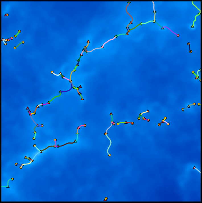
Another interesting post-treatment is the option -assemble that allows merging individual aligned pieces of filaments into larger structures. On the following picture, each piece of filament is represented with a distinct color:

M16_skelBST_nodes_fil.png

Running the following command (note once again that the order of arguments is important, try changing it ...):

skelconv m16_zo_no70um_density.fits_c4.2e+21.up.NDskl -breakdown -smooth 6 -trimBelow robustness 1.0E22 -assemble 70


one can assemble pieces of filaments that form an angle smaller than 70 degrees, resulting in the following structures, where individual pieces are straight but as long as possible:

M16_skelBSTA_nodes_fil.png


Point sample: 2D voids and filaments

This tutorial uses file ${DISPERSE}/data/simu_2D.ND which contains the projected distribution of the particles in a slice of an N-Body dark matter simulation of a 50 Mpc large chunk of the universe. Note that although we use a 2D slice for convenience here, the following procedure would also work with the full 3D distribution.

In this example, the voids and filaments of the particle distribution will be computed from the underlying density function traced by the particles, so we first need to define the topology of the space (i.e. we need a notion of neighborhood for each particle) and to estimate the density function. This is achieved using the Delaunay tessellation of the particle distribution, which can be computed with delaunay_2D.

The distribution of the particles is periodic, so we could simply run:

delaunay_2D simu_2D.ND -periodic


However, in this example we are going to pretend that the distribution has boundaries, which will make visualization easier (if boundary conditions are periodic, a filament crossing a boundary reappears on the other side, causing visual artifacts). We nevertheless would like to use the fact that boundary conditions are indeed periodic to correctly estimate density on the boundaries, which can be achieved using option -btype:

delaunay_2D simu_2D.ND -btype periodic


The output file is named simu_2D.ND.NDnet by default, and it contains the Delauany tessellation as an unstructured network in NDnet format, as well as the density function estimated using DTFE at each vertex (i.e. the additional vertex data labeled field_value in the NDnet file). This file can be fed directly to mse, but we have to choose a persistence threshold first.

Because the input file is a Delaunay tessellation, persistence is expressed as a ratio (density has a close to lognormal PDF) and the persistence threshold as a number of sigmas representing the probability that a persistence pair with given persistence ratio happens in a pure random discrete Poisson distribution. It is usually safe in such case to select a threshold between 2-sigmas and 4-sigmas, and we could directly compute the filaments of the distribution with the following command (see mse for more info):

mse simu_2D.ND.NDnet -nsig 3 -upSkl


However, in this example, we will use a persistence diagram to decide the correct threshold (in case you do not have pdview, replace -interactive with -nsig 3 in the following commannd) and we would also like to identify the voids in the distribution (i.e. the ascending 3-manifolds originating from critical points of critical index 0; see option -dumpManifolds of mse):

mse simu_2D.ND.NDnet -interactive -upSkl -dumpManifolds J0a


After running this command line, you should be able to visualize the following diagrams:

per_diag_small.jpg
On this picture, the maxima/saddle persistence pairs diagram is represented on the left and the minima/saddle one on the right. The fact that the second type of pairs are clearly less persistent reflects the known fact that dark matter haloes are very prominent structures because they belong to regions in the non linear regime where density increases exponentially fast. One nice feature of persistence diagrams is that they make it easy to choose the threshold above which underlying topological structures stand out of the noise : in the present case, we want to select the high persistence tails only that clearly stand out from the bunch of pairs generated by noise. This gives us a threshold of around 3-sigmas that can be visually selected by clicking while holding Ctrl key down. Once the threshold is selected, simply press Done button.

After this operation, mse should output two files: the filaments in a skeleton type file (simu_2D.ND.NDnet_s3.up.NDskl) and the voids in a network type file (simu_2D.ND.NDnet_s3_manifolds_J0a.NDnet).

By default, mse associates maxima to vertices while minima are associated to d-simplices (where d is the dimension of space). As a result, the network representing the voids defines a set of triangles each associated to a given void. This may not be very practical for post-treatment or visualization, but we can use option -vertexAsMinima to reverse the convention (this will overwrite the previous file if the threshold is identical):

mse simu_2D.ND.NDnet -nsig 3 -vertexAsMinima -dumpManifolds J0a


We can now visualize the result by converting the files to vtk formats using skelconv and netconv. The skeleton is smoothed and converted to vtp format:

skelconv simu_2D.ND.NDnet_s3.up.NDskl -smooth 10 -to vtp


and the input tesselation and output voids are converted to vtu format:

netconv simu_2D.ND.NDnet_s3_manifolds_J0a.NDnet -to vtu
netconv simu_2D.ND.NDnet -to vtu


the result should look as follows when visualized with paraview: (the configuration file ${DISPERSE}/data/simu_2D_nonper.pvsm can be directly loaded in paraview (File->Load State) to produce the following plot)

simu_2D_tuto_small.jpg

Note: on the right figure, a different color is associated to the source_index of each particle depending on which void it belongs to: each void originates from a different minimum of the field and each critical point has a specific index. This source_index corresponds to the position of this critical point as a node in skeleton files or as a vertex in persistence pair networks obtained with mse (options -dumpArcs and -ppairs). It can therefore also be used to cross-link information contained in manifold networks and skeletons or persistence pairs, such as for instance retrieving the hierarchy of the voids (i.e. using the parent_index of the critical points in skeleton files and persistence pairs networks).


Point sample: 3D walls and filaments

This tutorial follows the 2D discrete case example introduced in the previous section so you should probably read it first if you haven't done so yet.

We will compute the filaments and walls from the downsampled dark matter N-body simulation snapshot ${DISPERSE}/data/simu_32_id.gad. The distribution has periodic boundary conditions and we therefore start by computing its Delaunay tessellation with the following command:

delaunay_3D simu_32_id.gad -periodic


The program should output a file called simu_32_id.gad.NDnet that can be used directly with mse to compute the filaments and walls of the distribution. In 3D, walls are represented by the ascending 2-manifolds that originate from critical points of critical index 1 so they can be computed with option -dumpManifolds JE1a (letter E stands for Extended, which means that the ascending 1-manifolds and ascending 0-manifolds at the boundary of the walls will also be added, see option -dumpManifolds of mse) .Note that by default, subsets of the walls that are common to several walls are merged together, so you may want to try -dumpManifolds JP1a instead if you are interested in studying the properties of individual walls. The filaments are computed with option -upSkl or -dumparcs U which are equivalent. Using interactive mode to select a persistence threshold (use -nsig 3.5 instead of -interactive if pdview could not compile on your computer), we run the following command:

mse simu_32_id.gad.NDnet -dumpManifolds JE1a -upSkl -interactive


which after some quick computations, should display the following persistence diagram.

per_diag_3D.jpg
On this diagram, each type of pair is represented by a mark of different color : blue for minima/1-saddle, green for 1-saddle/2-saddle and red for 2-saddle/maxima. Note that the blue dots in the lower left corner stand for the voids in the distribution, so it is expected that we find only few of them compared to the red dots which represent collapsed structure (the simulation is 50 Mpc large). Each point on the diagram representing a topological feature, we would like to select only those points that stand out of the general distribution in terms of persistence in order to keep only the most meaningful structures (the persistence selection threshold is set by clicking while holding Ctrl key). The diagram suggests that persistence threshold should be above ~3-sigmas so we select a threshold of ~3.5 sigmas and click on the done button to confirm the selection. The program continues and should output the filaments in file simu_32_id.gad.NDnet_s3.52.up.NDskl and the walls in file simu_32_id.gad.NDnet_s3.52_manifolds_JE1a.NDnet.

It is instructive at that point to read mse output, and in particular the following section :

****** Simplifying complex ******
Starting Morse-Smale complex simplification.
Computing persistence pairs ... SKIPPED.
Sampling noise level was set to 3.5-sigma.
Cancelling pairs with persistance ratio < [2.66e+00,3.14e+00,4.42e+01].
   Tagging arcs ... done.
   Cancelling pairs (smart) ... (4140 rem.)
done.
   Cancellation took 0.10s (4140 canceled, 1 conflicts, 10 loops).


what mse tells us here is that it successfully removed 4140 persistence pairs, but was not able to cancel 11 more although their persistence was lower than the threshold. The 10 loops represent persistence pairs that were connected by more than one arc at the moment of their cancellation. Topologically speaking, their cancellation is not a valid operation as it would result in a discrete gradient loop (integral lines cannot form loops in Morse-theory). Note that the existence of non-cancellable pairs is not a bug of DisPerSE but rather a feature of Morse theory. However, not cancelling them may result in a few spurious non-significant pieces of filaments remaining in the ouput file (this is very problematic though as the impact on the identified filaments is very small in general) so one can use option -forceLoops to remove them anyway (which is perfectly fine if your goal is only to identify structures). Using this option will also solve the 1 conflict identified by mse, as conflicts are the result of a non-cancellable pair blocking the cancellation of a valid cancellable pair.

We can now rerun mse while skipping the computations by loading the backup file simu_32_id.gad.NDnet.MSC that mse generated on the previous run with option -loadMSC:

mse simu_32_id.gad.NDnet -dumpManifolds JE1a -upSkl -forceLoops -loadMSC simu_32_id.gad.NDnet.MSC -nsig 3.52


and the ouput should contain the following line:

   Cancellation took 0.10s (4151 canceled, 0 conflicts, 11 forced loops).


indicating that all the 4151 non persistent pairs could be cancelled.

We can now smooth and convert the resulting files to a more portable format:

skelconv simu_32_id.gad.NDnet_s3.52.up.NDskl -smooth 10 -to vtp
netconv simu_32_id.gad.NDnet -to vtu
netconv simu_32_id.gad.NDnet_s3.52_manifolds_JE1a.NDnet -smooth 10 -to vtu


and visualize the result with paraview. The configuration file ${DISPERSE}/data/simu_32_per.pvsm can be directly loaded in paraview (File->Load State) to make the following plot: (note that it is a bit tricky to deal with periodic boundary conditions when visualizing, clipping the boundaries is usually the easiest way)

simu_3D_result_small.jpg

Note: contrary to the previous example where we computed 2D voids (see here), it is problematic in this case to identify each individual wall and paint it with a specific color. Indeed, contrary to voids, the 2-manifolds that represent walls can overlap, and so a unique source_index representing the critical point from which each wall originates cannot be assigned to each simplex (i.e. in that case, triangle). A solution to this problem would have been to specify that we wanted identical simplices to be stored as many times as they appear in different walls even though they are the same. This could have been achieved with flag P of option -dumpManifolds in mse:

mse simu_32_id.gad.NDnet -dumpManifolds JEP1a -upSkl -forceLoops -loadMSC simu_32_id.gad.NDnet.MSC -nsig 3.52


As a result, the output file is larger, but it would also allow cross-linking the information contained in the geometry of the walls and that in the skeleton files or persistence pairs network (see this note).