This program is distributed freely for non-commercial use, however, we ask users to kindly cite DisPerSE as appropriately as possible in their papers, in particular by referencing the following articles (Sousbie 2011 and Sousbie & al. 2011):
@ARTICLE{2011MNRAS.414..350S,
author = {{Sousbie}, T.},
title = "{The persistent cosmic web and its filamentary structure - I. Theory and implementation}",
journal = {\mnras},
archivePrefix = "arXiv",
eprint = {1009.4015},
primaryClass = "astro-ph.CO",
keywords = {methods: data analysis, methods: numerical, galaxies: formation, galaxies: kinematics and dynamics, cosmology: observations, large-scale structure of Universe},
year = 2011,
month = jun,
volume = 414,
pages = {350-383},
doi = {10.1111/j.1365-2966.2011.18394.x},
adsurl = {http://adsabs.harvard.edu/abs/2011MNRAS.414..350S},
adsnote = {Provided by the SAO/NASA Astrophysics Data System}
}

@ARTICLE{2011MNRAS.414..384S,
author = {{Sousbie}, T. and {Pichon}, C. and {Kawahara}, H.},
title = "{The persistent cosmic web and its filamentary structure - II. Illustrations}",
journal = {\mnras},
archivePrefix = "arXiv",
eprint = {1009.4014},
primaryClass = "astro-ph.CO",
keywords = {methods: data analysis, galaxies: formation, galaxies: kinematics and dynamics, cosmology: observations, dark matter, large-scale structure of Universe},
year = 2011,
month = jun,
volume = 414,
pages = {384-403},
doi = {10.1111/j.1365-2966.2011.18395.x},
adsurl = {http://adsabs.harvard.edu/abs/2011MNRAS.414..384S},
adsnote = {Provided by the SAO/NASA Astrophysics Data System}
}
You can download the latest version of the source code here (V0.9.23) : disperse_latest.tar.gz
Go to the ${DISPERSE_SRC}/build directory and type:
cmake ../
This will check the configuration and generate the Makefile. Read the output to know which library were found, which were not, and how to specify their path (option -DLIBNAME_DIR=path/to/library/ where {LIBNAME} may be QT,GSL,SDL,MATHGL or CGAL).
The default install path is "${DISPERSE_SRC}", but it can be changed using option -DCMAKE_INSTALL_PREFIX=PATH/TO/INSTALL/DIR. Then just compile and install with:
make install -j N
where N is the number of processors to be used for compilation. One to seven executables should be created in ${DISPERSE_SRC}/bin (or ${CMAKE_INSTALL_PREFIX}/bin if set), depending on which libraries were found:
DisPerSE stands for Discrete Persistent Structures Extractor and its main purpose is to identify persistent topological features such as peaks, voids, walls and in particular filamentary structures within sampled distributions in 2D, 3D, and possibly more ...
Although it was initially developed with cosmology in mind (for the study of the properties of filamentary structures in the so called comic web of galaxy distribution over large scales in the Universe), the present version is quite versatile and should be useful for any application where a robust structure identification is required, for segmentation or for studying the topology of sampled functions (like computing persistent Betti numbers for instance).
DisPerSE is able to deal directly with noisy datasets using the concept of persistence (a measure of the robustness of topological features) and can work indifferently on many kinds of cell complex (such as structured and unstructured grids, 2D manifolds embedded within a 3D space, discrete point samples using delaunay tesselation, Healpix tesselations of the sphere, ...). The only constraint is that the distribution must be defined over a manifold, possibly with boundaries.
In DisPerSE, structures are identified as components of the Morse-Smale complex of an input function defined over a - possibly bounded - manifold. The Morse-Smale complex of a real valued so-called Morse function is a construction of Morse theory which captures the relationship between the gradient of the function, its topology, and the topology of the manifold it is defined over.
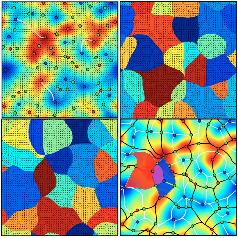
Figure 1: the Morse-Smale complex
Two central notions in Morse theory are that of critical point and integral line (also called field line) : (see the upper left frame of figure 1)
-Critical points are the discrete set of points where the gradient of the function is null. For a function defined over a 2D space, there are three types of critical points (4 in 3D, ...), classified by their critical index. In 2D, minima have a critical index of 0, saddle points have a critical index of 1 and maxima have a critical index of 2. In 3D and more, different types of saddle points exist, one for each non extremal critical index.
-Integral lines are curves tangent to the gradient field in every point. There exist exactly one integral line going through every non critical point of the domain of definition, and gradient lines must start and end at critical points (i.e. where the gradient is null).
Because integral lines cover all space (there is exactly one critical line going through every point of space) and their extremities are critical points, they induce a tessellation of space into regions called ascending (resp. descending) k-manifolds where all the field lines originate (respectively lead) from the same critical point (see ascending and descending 2-manifolds on figure 1, upper right and lower left panels). The number of dimensions k of the regions spanned by a k-manifold depend directly on the critical index of the corresponding critical point: descending k-manifolds originate from critical points of critical index k while the critical index is N-k for ascending manifolds, with N the dimension of space.
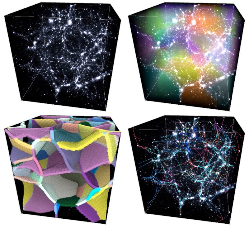
The set of all ascending (or descending) manifolds is called the Morse complex of the function. The Morse-Smale complex is an extension of this concept: the tessellation of space into regions called p-cells where all the integral lines have the same origin and destination (see figure 1, lower right frame). Each p-cell of the Morse-Smale complex is the intersection of an ascending and a descending manifold and the Morse-Smale complex itself is a natural tessellation of space induced by the gradient of the function. Figure 2 below illustrates how components of the Morse-Smale complex can be used to identify structures in a 3D distribution.
Figure 2: 3D structures identified as component of the Morse-Smale complex
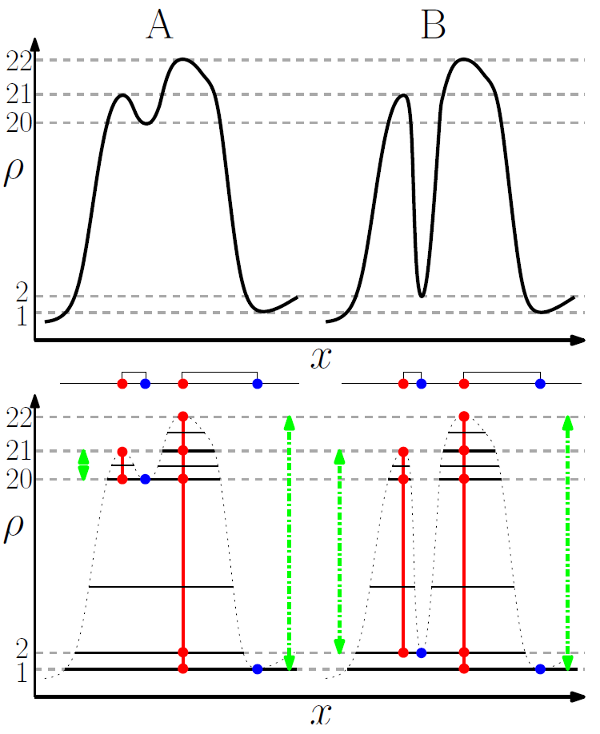
Persistence itself is a relatively simple but powerful concept. To study the topology of a function, one can measure how the topology of its excursion sets (i.e. the set of points with value higher than a given threshold) evolves when the threshold is continuously and monotonically changing. Whenever the threshold crosses the value of a critical point, the topology of the excursion change. Supposing that the threshold is sweeping the values of a 1D function from high to low, whenever it crosses the value of a maximum, a new component appears in the excursion, while two components merge (i.e. one is destroyed) whenever the threshold crosses the value of a minimum. This concept can be extended to higher dimensions (i.e. creation/destruction of hole, spherical shells, ....) and in general, whenever a topological component is created at a critical point, the critical point is labeled positive, while it is labeled negative if it destroys a topological component. Using this definition, topological components of a function can be represented by pairs of positive and negative critical points called persistence pairs. The absolute difference of the value of the critical points in a pair is called its persistence : it represents the lifetime of the corresponding topological component within the excursion set.
Figure 1: Persistence pairs
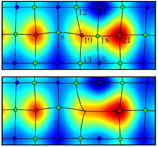
The concept of persistence is powerful because it yields a simple way to measure how robust topological components are to local modifications of a function values. Indeed, noise can only affect a function's topology by creating or destroying topological components of persistence lower that its local amplitude. Therefore, it suffice to know the amplitude of noise to decide which components certainly belong to an underlying function and which may have been affected (i.e. created or destroyed) by noise. In DisPerSE, a persistence threshold can be specified (see options -nsig and -cut of mse) to remove topological components with persistence lower than the threshold and therefore filter noise from the Morse-Smale complex (see figure 2 below).
Figure 1: Morse-smale complexsimplification
A very useful way to set the persistence threshold is to plot a persistence diagram, in which all the persistence pairs are represented by points with coordinates the value at the critical points in the pair (see option -interactive of mse or see pdview and read the tutorial section to learn how to compute and use persistence diagrams).
In DisPerSE, the different types of cells that compose the Morse-Smale complex are used to identify different types of structures. In this document, we adopt the following terminology:
- A critical point is a point where the gradient is null. In N dimensional space, there are N types of critical point, characterized by a critical index.
- A maximum is a critical point of critical index N in an N dimensional space.
- A minimum is a critical point of critical index 0.
- A k-saddle point is a critical point of critical index k that is neither a minimum nor a maximum.
- A d-simplex is the most simple geometrical figure in d dimensions and consists of d+1 points linked together (i.e a point, segment, triangle, tetrahedron ... for d=0,1,2,3,...). In DisPerSE, space is decomposed into d-simplices and each critical point is associated to a given d-simplex (by default, maxima are 0-simplices, saddle-points are 1-simplices, ...).
- A persistence pair is a pair of critical points with critical index difference of 1. A persistence pair represents a topological component of the function. More details here.
- Persistence is defined as the difference (or ratio) of the value at the two critical points in a persistence pair. Persistence is always positive and represents the importance of the topological feature defined by the persistence pair : low persistence pairs are sensible to changes in the value of the function, and the corresponding critical points are easily destroyed, even by small perturbations, while high persistence pairs are robust. Removing low persistence pairs from the Morse-Smale complex is a good way to filter noise and/or non-meaningfull structures. More details here.
- Robustness is a local measure of how contrasted the critical points and filaments are with respect to their background. In a sense, robustness is a continuous version of persistence which extends to filaments (persistence applies to pairs of critical points only). What we call robustness here is actually an improved version of the separatrix persistence described in Weinkauf, T. and Gunther, D., 2009. See options -trimBelow of skelconv, -robustness of mse and the tutorial section for more details and possible applications.
- An integral line is a curve tangent to the gradient field in every point. There exist exactly one integral line going through every non critical point of the domain of definition, and gradient lines must start and end at critical points (i.e. where the gradient is null).
- A descending k-manifold is a k dimensional region of space defined as the set of points from which following minus the gradient leads to the same critical point of critical index k, with N the dimension of the space (e.g. a descending N-manifold originates from a maximum). More details here.
- An ascending k-manifold is a k dimensional region of space defined as the set of points from which following the gradient leads to the same critical point of critical index N-k, where N is the dimension of the space (e.g. an ascending N-manifold originates from a minimum). More details here.
- A Morse p-cell is a p-dimensional region of space defined by the intersection of an ascending and a descending manifold. All Integral lines in a morse p-cell originate and lead to the same critical points. More details here.
- A Morse-Smale complex of a Morse function is the tessellation of space induced by its gradient : it divides space into regions where the integral lines originate from and lead to the same critical points. Its elements are the Morse p-cells. More details here.
- An arc is a Morse 1-cell : a 1D curve traced by the integral line that joins two critical points together. There is always exactly two arcs originating from a saddle point and leading to an extremum (i.e. a minimum or a maximum). In 3D and more however, the number of arcs linking two saddle point together is arbitrary. More details here.
- A skeleton is a set of arcs. We call upper-, lower-, and inter- skeleton the set of arcs that lead or originate from exactly one maximum, exactly one minimum, or none of the two respectively.
- A filament is a 1-dimensional structure : an ascending or descending 1-manifold. A filament consists of the set of two arcs originating from a given saddle point and joining two extrema together (i.e. the yellow+green arcs on lower right frame of figure 1). Unless explicitly stated, filaments join maxima together and we sometime call void filaments or anti-filaments the filaments that link minima together.
- A wall is a 2-dimensional structure : an ascending or descending 2-manifold. Walls exist only in 3D and more and delimit the voids or peak patches.
- A void is a N dimensional structure (N being the dimension of space): an ascending N-manifold that originates from a given minimum of the field. A void is the set of points from which following the gradient leads to a given minimum.
- A peak patch is a N dimensional structure (N being the dimension of space): a descending N-manifold that originates from a given maximum of the field. Peak patches are the dual of voids: the set of points from which following the opposite of the gradient leads to the same maxima.
mse is the main program in DisPerSE, it is used to compute Morse-smale complexes and extract filamentary structures (i.e. arcs), voids and walls (ascending/descending manifolds), critical points and persistence pairs. By default, when no option is specified, the Morse-smale complex is computed and stored as a filename.MSC backup file in a format internal to mse, and no other file is produced. This file may later be loaded by mse (option -loadMSC) to skip the computation of the Morse-smale complex (this is useful when you want to produce different outputs from the same source).
The cell complex defining the topology of the space and optionally the function discretely sampled over it. The file may be a Healpix FITS file, a regular grid or an unstructured network readable by netconv or fieldconv (run netconv or fieldconv without argument for a list of supported file formats). The value of the function from which the Morse-smale complex will be computed should be given for each vertex (or pixel in case of a regular grid). In the case of an unstructured network, the function should be given in a field labeled field_value, or the function may also be set using option -field.
-field <fname>:
Specifies the scalar function whose morse complex will be computed. The function value should be given for each vertex (or pixel for regular grids), so the file must be a 1D array of values of size the number of vertices (or pixels) in the network, in a readable grid format.
-outName <fname>:
Specifies the base name of the output file (extensions are added to this base name depending on the output type). Default value: the name of the input network file.
-outDir <dir>:
Specifies the output directory. Default value: the current working directory.
-noTags:
Prevents mse from adding trailing extensions to the output filename such as the persistence cut levels ... Note that the last extension correponding to the file format is still added.
-periodicity <val>:
Specifies the periodicity of the domain. This is only applicable to grid types networks, which are considered by default to have periodic boundaries. The parameter <val> is a serie of 1s and 0s enabling/disabling periodic boundary conditions along the corresponding direction. Exemple: -periodicity 0 sets non periodic boundaries conditions (PBC) while -periodicity 101 sets PBC along dims 0 and 2 (x and z) but not along y axis. Default value: by default, boundary conditions are fully periodic.
-mask <fname> [~]:
Specifies a mask. The file must be a 1D array of values of size the number of vertices (or pixels) in the network, in a readable grid format. By default, a value of 0 corresponds to a visible vertex/pixel while any other value masks the vertex/pixel. Adding a trailing ~ to the filename (without space) reverses this behavior, a value of 0 masking the corresponding pixels/vertices.
-nthreads <N=$OMP_NUM_THREADS>:
Specifies the number of threads. Default value: the number of threads is set by the environment variable $OMP_NUM_THREADS which is usually set to the total number of cores available by openMP.
-nsig <n1, n2, ...>:
Specifies the persistence ratio threshold in terms of "number of sigmas". Any persistence pair with a persistence ratio (i.e. the ratio of the values of the points in the pair) that has a probability less than "n-sigmas" to appear in a random field will be cancelled. This may only be used for discretely sampled density fields (such as N-body simulations or discrete objects catalogs) whose density was estimated through the DTFE of a delaunay tesselation. This option is typically used when the input network was produced using delaunay_2D or delaunay_3D, in any other case, use -cut instead. See also option -interactive
-cut <l1, l2, ...>:
Specifies the persistence threshold. Any persistence pair with persistence (i.e. the difference of value between the two points in the pair) lower than the given threshold will be cancelled. Use -nsig instead of this when the input network was produced with delaunay_2D or delaunay_3D. The cut value should be typically set to the estimated amplitude of the noise. See also option -interactive.
-interactive [<full/path/to/pdview>]:
This option allows the user to interactively select the persistence threshold on a persistence diagram (using pdview). if option -cut or -nsig is also used, the specified values are become default thresholds in pdview. The path to pdview may be optionally indicated in case it cannot be found automatically. Note: this option may only be used if pdview was compiled (requires mathGL and Qt4 libraries).
-forceLoops:
Forces the simplification of non-cancellable persistence pairs (saddle-saddle pairs in 3D or more that are linked by at least 2 different arcs). When two critical points of critical index difference 1 are linked by 2 or more arcs, they may not be cancelled as this would result in a discrete gradient loop. This is not a problem in 2D as such pairs cannot form persistence pairs but in 3D, saddle-saddle persistence pairs may be linked by 2 or more arcs even though their persistence is low. By default those pairs are skipped in order to preserve the properties of the Morse-smale complex but as a result few non persistent features may remain (such as spurious filaments). Fortunately, there are usually none or only very few of those pairs, and their number is shown in the output of mse, in the Simplifying complex section. If you are only interested in identifying structures (as opposed to doing topology), you should probably use '-forceLoops' to remove those spurious structures (such as small non significant filaments).
-robustness / -no_robustness:
Enables or prevents the computation of robustness and robustness ratio. By default, robustness is not computed as it can be costly for very large data sets. When enabled, a robustness value is tagged for each segments and node of the output skeleton files. See also options -trimBelow of skelconv and the tutorial section for applications.
-manifolds:
Forces the computation and storage of all ascending and descending manifolds (i.e. walls, voids, ...). By default, mse only stores manifolds geometry if required (for instance, when the option -dumpManifolds is used), and the resulting backup MSC file will therefore not contain this information and may not be used later to compute manifolds. Example: running the command 'mse filename' will produce a the backup file 'filename.MSC' that stores the Morse-smale complex information. A later call to mse -loadMSC filename.MSC -upSkl would skip the computation of the MS-complex and succeed in producing the skeleton of the filamentary structures (arcs) as arcs geometry is computed by default. Unfortunately, mse -loadMSC filename.MSC -dumpManifolds J0a would fail as the information needed to compute the ascending 3-manifolds (i.e. manifolds originating from a minimum, which trace the voids) is not avaialble by default. Running mse filename -manifolds in the beginning would solve this problem.
-interArcsGeom:
This is similar to option -manifolds, but for the arcs linking different types of saddle-points together (in 3D or more). By default, unless option -interSkl is specified, only the geometry of arcs linking extrema to saddle points is computed, so the backup .MSC file may not be used later to retrieve other types of arcs geometry. Specifying -interArcsGeom forces the computation and storage of all types of arcs in the .MSC backup file.
-no_arcsGeom:
By default, the geometry of arcs linking extrema and saddle point is always computed even when not directly needed, so that it is stored in the backup .MSC file for later use. Specifying -no_arcsGeom may be used to lower memory usage when only the critical points and/or their persistence pairings are needed. Exemple: mse filename -ppairs -no_arcsGeom will compute the critical points and persistence pairs using less memory than mse filename -ppairs, but the resulting .MSC file may not be later used to retrieve arcs geometry.
-ppairs:
Dumps the persistence pairs as a NDnetnetwork type file. The resulting file is a 1D network, where the critical points are the vertices and 1-cells (segments) represent pairs. Additional information such as the type, persistence, cell in the initial complex, ... of each critical points and pairs is also stored as additional information. Try running netconv filename.ppairs.NDnet -info for a list of available additional data (see also additional data in the network file format section).
-ppairs_ASCII:
Same as -ppairs but pairs are dumped in a easily readable ASCII format. This option is deprecated and should not be used, use -ppairs option instead and then run netconv filename.ppairs.NDnet -to NDnet_ascii.
-upSkl:
Dumps the "up" skeleton (i.e. arcs linking maxima to saddle-points, which trace the filamentary structures) as a NDskl type skeleton file. This command is an alias of -dumpArcs U.
-downSkl:
Dumps the "down" skeleton (i.e. arcs linking minima to saddle-points, which trace the anti-filaments, or void filaments) as a NDskl type skeleton file. This command is an alias of -dumpArcs D.
-interSkl:
Dumps the "inter" skeleton (i.e. arcs linking different types of saddle-points together) as a NDskl type skeleton file. This will only work in 3D or more, and be careful that those type of arcs may have a very complex structure. This command is an alias of '-dumpArcs I''.
-dumpArcs <CUID>:
Dumps the specified type of arcs (i.e filaments) as a NDskl type skeleton file. Any combination of the letter C, U, I and D may be used as parameter to indicate which type of arc should be saved:
-D(own): arcs leading to minima (see also -downSkl).
-I(nter): other arcs linking saddle-points together (see also -interSkl).
-C(onnect): keeps at least the connectivity information for all types of arcs.
Exemple: CUD dumps geometry of arcs for which one extremity is and extremum (a maximum or a minimum), and the connectivity of saddle points is also stored (i.e. one can retrieve how they are linked in the Morse-Smale complex but not the actual geometry of the corresponding arcs).
-dumpManifolds [<JEP0123456789ad>]:
Dumps ascending and/or descending manifolds (i.e. walls, voids, ...) as a NDnet type network file. The first part of the argument must be a combination of letters J, E and P and the second, which indicates the type of manifold to dump as a digit indicating the critical index of the critical point it originates from followed by the letter a and/or d to select ascending and/or descending manifolds respectively:
- J(oin): join all the the manifolds in one single file. By default, one file is created for each manifold.
- E(xtended): compute extended manifolds. For instance, when computing an ascending 2-manifold (i.e. a wallseparating two voids), the ascending 1-manifolds (i.e. filaments) on its boundary as well as the ascending 0-manifolds (i.e. critical points) on their boundaries are also dumped.
- P(reserve): do not merge infinitely close submanifolds. By default, the overlapping part of manifolds are merged (e.g. filaments may have bifurcation points but arcs only stop at critical points, so although two arcs continue above the bifurcation, only one path is stored). Using this option preserve the properties of the MS-complex but may result in very large files.
- D(ual): compute dual cells geometry when appropriate. Descending and ascending manifolds are the dual of one another, so they should be represented by cells of the complex and their dual respectively. When this option is used, appropriate cells are replaced by their dual (for instance, ascending 0-manifolds of a delaunay tesselation are represented by sets of voronoi 3-cells, the dual of the 0-cells (vertices) of the delaunay tesselation). The default behavior is that descending manifolds belong to the dual, so ascending manifolds are always fine but one may want to use option D to compute dual cells or option -vertexAsMinima to change this behavior in order to obtain correct descending manifolds.
- 0123456789: specifies the critical index of the critical points from which the manifold originates (ascending 0,1,2 and 3-manifolds in 3D trace the voids, walls, filaments and maxima/sources respectively).
- a/d: compute the ascending and/or descending manifold.
Exemple 1: in 3D, argument JD0a2ad3d would dump to a single file the ascending manifolds of critical index 0 and 2, and the descending ones for critical index 2 and 3. Cells are replaced by their dual where appropriate (i.e. in 3D, the descending 2-manifolds would be 2-cells dual of segments, and descending 3 manifolds would be 3-cells dual to vertices).
Exemple 2: in 3D, argument JE0a would dump the union of the tetrahedrons within the voids, the walls separating the voids, as well as the filaments on their boundaries and the maxima at their extremity, as sets of triangles, segments and vertices of the input complex respectively, to a single file. As option P was not used, any overlapping region would be stored only once.
-compactify <type=natural>:
This option is used to specify how to treat boundaries of manifolds with boundary (this option does not affect manifolds without boundary). Available type are:
- 'natural' is the default value, and almost always the best choice.
- 'sphere' links boundaries to a cell at infinity.
-vertexAsMinima:
As mse uses discrete Morse theory, each type of critical point corresponds to a particular cell type. By defaults, 0-cells (vertices) are maxima, 1-cells are saddle points, .... and d-cells are minima (d is the number of dimensions). Using -vertexAsMinima, the association is reversed and 0-cells are associated to minima ... while d-cells are associated to maxima. This option can be useful to identify manifolds or arcs as lists of a particular type of cell. Example: mse input_filename -dumpManifolds J0a -vertexAsMinima can be used to identify voids (ascending 0-manifolds) as sets of 0-cells (vertices). As a result, voids are identified as sets of pixels or particles (if input_filename is a grid or the delaunay tesselation of an N-body simulation respectiveley), which is easy to relate to the pixels/particles of the input file. If the command mse input_filename -dumpManifolds J0a had been issued instead, each void would have been described by a set of n-cells (in nD).
-descendingFiltration:
By default, mse uses an ascending filtration to compute the discrete gradient. This option forces the program to use a descending filtration instead. Not that if mse works correctly (and it should hopefully be the case) the general properties of the Morse-smale complex are not affected, but simply critical points and manifolds geometry will slightly differ.
-no_saveMSC:
Use this if you do not want mse to write a backup .MSC file.
-loadMSC <fname>:
Loads a given backup .MSC file. This will basically skip the computation of the Morse-smale complex, therefore gaining a lot of time. By default, mse always write a backup .MSC after the MS-complex is computed. See options -manifolds and -interArcsGeom for information on the limitations.
-no_gFilter:
Prevents the filtration of null-persistence pairs in the discrete gradient. There is no point in using this option except for debugging ...
-diagram:
Draws a diagram of the connectivity of critical points to a .ps file. This should only be used when the number of critical points is very small (i.e. less than 100 or so).
-smooth <Ntimes=0>:
Deprecated, don't use it ... use skelconv -smooth <Ntimes=0> or netconv -smooth <Ntimes=0> on the output files instead.
Delaunay_2D and Delaunay_3D are used to compute the Delaunay tessellation of a discrete particle distribution (such as a N-Body simulation or a catalog of object coordinates) in 2D and 3D respectively and possibly in parallel. The output is an unstructured network in NDnet format, with density computed for each vertex using DTFE (i.e. density at a given vertex is proportional to the total volume of the surrounding cells). In order to compute the correct topology and density close to the boundaries, the distribution is extrapolated over a band outside the domain of definition (see options -margin, -btype and -periodic). The output network can be used as input file for mse to compute the Morse-Smale complex of the initial discrete sample (the index of the vertices in the output network correspond to the index of the sampling particles in the input file).
The name of a file containing the discrete particle coordinates in a field format.
-outName <fname>:
Specifies the base name of the file in output (extensions are added to this base name depending on the output type). Default value: the name of the input file.
-outDir <dir>:
Specifies the output directory. Default value: the current working directory.
-subbox <x0> <y0> [<z0>] <dx> <dy> [<dz>]:
Restricts the computation to a box of size [dx dy dz] and with origin [x0,y0,z0]. The box may be larger than the actual bounding box or cross its boundaries. The distribution outside the box will depend on the boundary type, as set with option -btype. Note that the distribution within the margin of the subbox (see option -margin) is still used to compute the topology close to the boundaries, so this option may be used to cut a large distribution into several small sub-boxes with matching boundary distribution.
-periodic:
Use this option to force periodic boundary conditions for the output network. When this option is used, delaunay_nD will try to reconnect the simplices crossing the bounding box so that the space is compactified to a torus. The operation may fail if the margin size is too small, as cells crossing opposite boundaries may not match, so always check the output of the program as an estimation of the correct margin size will be indicated in that case (see also option -margin). Note that this option wil set default boundary type to -btype periodic.
-minimal:
when using this option, only the minimal necessary information to define the tesselation is stored in the output file (i.e. In dimensions D, the vertex coordinates and simplices of dimension D, and the additional data associated to them). Note that it is preferable NOT to use this option when the ouput file is to be fed to mse, as it will force the program to recompute the topology of intermediate simplices using a slower algorithm every time it is run.
-blocks <NChunks> <NThreads>:
instead of computing the delaunay tesselation of the full distribution, divide it into NChunks overlapping sub blocks and process them NThreads at a time. The subblocks are then automatically reassembled into the full delaunay tesselation. This option can either be used to increase speed by parallelizing the process (for high values of NThreads) or decrease the memory consumption (when NChunks>>NThreads). Note that it is incompatible with options -mask, -btype smooth, -angmask and -radialDensity.
-margin <M>:
Suggests a startup trial size for the additional margin used to compute the topology and density close to the boundary. The margin size is expressed as a fraction of the bounding box (or subbox if option -subbox is used). Note the the program can probably make a better guess than you so it is not recommanded to set it by hand ...
-btype <t=mirror>:
This option sets the type of the boundaries. This option is used to set how the distribution should be extrapolated outside the bounding box (an estimation of the distribution outside the bounding box is needed to correctly estimate the topology and density of the distribution close to its boundaries). Possible boundary types are:
- mirror : the distribution outside the bounding box is a mirrored copy of that inside.
- periodic : use periodic boundary condition (i.e. space is paved with copies of the distribution in the bounding box). Note that this option does *NOT* enforce periodic boundary conditions as it does not tell delaunay_nD to reconnect the Delaunay cells that cross the bounding box (this is achieved with -periodic).
- smooth : a surface of guard particles is added outside the bounding box and new particles are added by interpolating the estimated density computed on the boundary of the distribution. This boundary type is useful when the actual boundaries of the sample are complex (i.e. not a cube), such as for a 3D galaxy catalog limited to a portion of the sky.
- void : the distribution is supposed to be void outside the bounding box.
-mask <fname.ND>:
Specifies a mask. The file must be a 1D array of values of size the number of vertices (or pixels) in the network, in a readable grid format. A value of 0 corresponds to a non-masked particle while any other value masks the particle. Note that masked particles are still used to compute the Delaunay tessellation and estimate the density but they will change the topology of the actual distribution.
-smooth <N=0>:
Smooth the estimated DTFE density by averaging N times its value at each vertex with that at the neighboring vertices (i.e two vertices are considered neighbors if they both belong to the boundary of at list one given cell).
pdview is used to interactively select the persistence threshold with the help of a persistence diagram. A persistence diagram is a 2D plot in which all the persistence pairs are represented by points with coordinates the value at the critical points in the pair (see this section for more info). In pdview, we rather represent the value of the lower critical index on the x axis and the absolute difference in value between the two critical points on the y axis (i.e. the persistence of the pair). The diagram is computed from a network file encoding the persistence pairs as output by mse filename -ppairs. Press the button labeled ? in pdview for more information on how to use it.
netconv is used to post-treat, convert and display information about unstructured network format files. Run netconv without argument to see a list of available input and output formats.
The name of a file containing an unstructured network (for instance, persistence pairs or manifolds as output by mse) in a readable network file format.
-outName <fname>:
Specifies the base name of the output file (extensions are added to this base name depending on the output type). Default value: the name of the input file.
-outDir <dir>:
Specifies the output directory. Default value: the current working directory.
-addField <filename> <field_name>:
Tags each vertex of the network with the interpolated value of a field. The parameter filename is the name of a readable regular grid field format file containing the grid to be interpolated, and field_name is the name of the additional field in the output file.
-smooth <Ntimes=0>:
Smooth the network N times. Smoothing is achieved by averaging the position of each vertex with that of its direct neighbors (i.e. those that belong to the boundary of at least one common simplex). In practice, smoothing N times makes the network smooth over the local size of '~N' network cells. Smoothing is first achieved only on vertices sharing at least a common 3-simplex, then a 2-simplex, ... So for instance when smoothing manifolds such as output by mse -dumpManifolds JE0a, walls will be smoothed independently of filaments and critical points (try it yourself to understand ...).
-smoothData <vertex_field_name> <Ntimes>:
smooth the vertex_field_name data field associated with vertices by averaging its value with that of its direct neighbors in the network Ntimes times.
-noTags:
Prevents netconv from adding trailing extensions to the output filename. Note that the last extension correponding to the file format is still added.
-toRaDecZ:
Converts the coordinates to Ra (Right ascension), Dec (Declination) and Z (redshift). This is useful when the input file was computed from a particle distribution whose coordinates where given in the same system (such as a galaxy catalog for instance, see catalog format in field format).
-toRaDecDist:
Converts the coordinates to Ra (Right ascension), Dec (Declination) and Dist (Distance). This is useful when the input file was computed from a particle distribution whose coordinates where given in the same system (such as a galaxy catalog for instance, see catalog format in field format).
-info:
Prints information on the input file, such as the number of each type of cell and the name and type of additional fields.
-to <format>:
Outputs a file in the selected writable unstructured network format. A list of possible parameter values can be obtained by running netconv without any argument.
skelconv is used to post-treat, convert and display information about skeleton format files. Run skelconv without argument to see a list of available input and output formats. Note that skeleton files can also be converted to NDnet format unstructured networks readable by netconv.
nb: in skelconv, the order of the argument on the command line is important and certain post-treatment do not commute. In particular, be careful when using options -breakdown, -trim, -smooth or -assemble together as for instance -smooth 3 -breakdown or -breakdown -smooth 3 will not produce the same output.
The name of a file containing a skeleton such as skeletons (filaments) output by mse in a readable skeleton format.
-outName <fname>:
Specifies the base name of the output file (extensions are added to this base name depending on the output type). Default value: the name of the input file.
-outDir <dir>:
Specifies the output directory. Default value: the current working directory.
-noTags:
Prevents skelconv from adding trailing extensions to the output filename. Note that the last extension correponding to the file format is still added.
-smooth <Ntimes=0>:
Smooth the skeleton N times. When using this option, the nodes (i.e. critical points) are fixed and the filaments are smoothed by averaging the coordinates of each points along a filament with that of its two neighbors. Smoothing N times effectively make filaments smooth over ~N sampling points.
-breakdown:
By default, skeletons are composed of arcs linking critical points together, so an arc will always start and stop at a critical point. Different arcs with same destination may partially overlap though, between a so-called bifurcation and a critical point. If N arcs overlap in a given place, the N segments will describe their geometry in that place : this is topologically correct but may not be desirable when computing statistics along the filaments as it would artificially increase the weight of those regions. Using -breakdown, bifurcation points are replaced by fake critical points with critical index D+1 (where D is the number of dimensions), and infinitely close pieces of arcs are merged. This option should most probably be used before computing any statistical quantity along arcs ...
-assemble [[<field_name>] <threshold>] <angle>:
Assemble arcs into longer filaments, with the constraint that they do not form an angle larger than <angle> (expressed in degrees) and optionally do not go below threshold <threshold> in the field <field_name>. See option -trim for explanations on the first two arguments. When using this option, the algorithm will try to find the longest possible aligned arcs and will join them, removing critical points and creating only straight filaments. Option -breakdown should almost always be used before using this (e.g. skelconv filename.NDskl -breakdown -assemble 0 45).
-trimAbove/trimBelow [<field_name>] <threshold>:
Trims the regions of the skeleton above or below threshold <threshold> and add nodes (fake critical points of index D+1) at the extremity of trimmed arcs. By default, the skeleton is trimmed according to field_value (i.e. the value of the function from which the skeleton was computed). One can specify a different function with <field_name> (a list of possible fields may be obtained running skelconv filename.NDskl -info). One particularly interesting trimming function is robustness which is an extension of the concept of persistence to each points of the arcs ( an improved version of the separatrix persistence described in Weinkauf, T. and Gunther, D., 2009 ). Indeed, robustness can be considered a measure of how contrasted the filament is with respect to its local background, and it is therefore a good way to select only highly contrasted subsets of the filamentary structures. Note that robustness, like persistence, is defined as a difference or ratio between the value of the field in two points, so the robustness threshold has the same order of magnitude as the persistence threshold.
-toRaDecZ:
Converts the coordinates to Ra (Right ascension), Dec (Declination) and Z (redshift). This is useful when the input file was computed from a particle distribution whose coordinates where given in the same system (such as a galaxy catalog for instance, see catalog format in field format).
-toRaDecDist:
Converts the coordinates to Ra (Right ascension), Dec (Declination) and Dist (Distance). This is useful when the input file was computed from a particle distribution whose coordinates where given in the same system (such as a galaxy catalog for instance, see catalog format in field format).
-rmBoundary:
Remove the arcs and nodes that lay on the boundary or outside the domain of definition (e.g. nodes/arcs at infinity generated by boundary conditions).
-rmOutside:
Remove the artificial arcs and nodes generated by the boundary conditions (e.g arcs/nodes at infinity) but keep boundaries (this is less restricitve than -rmBoundary).
-toFITS [<Xres>] [<Yres>] [<Zres>]:
Samples the skeleton to a FITS image with specified resolution. If the resolution is omitted (parameters Xres, Yres and/or Zres), then the output file will have the same resolution as the network that was used to compute the skeleton.
-info:
Prints information on the input file, such as the number of arcs, critical points and the name and type of additional fields.
-addField <filename> <field_name>:
Tags each segment (i.e. pieces of arcs) and node (i.e. critical point) of the skeleton with the interpolated value of a field. The parameter filename is the name of a readable regular grid field format file containing the grid to be interpolated, and field_name is the name of the additional field in the output file.
-to <format>:
Outputs a file in the selected writable skeleton format. A list of possible parameter values can be obtained by running skelconv without any argument. Note that skeleton files can be converted to NDnet format unstructured networks readable by netconv.
fieldconv is used to display information about field format files encoding regular grid or point set coordinates, and convert them to other formats. Run fieldconv without argument to see a list of available input and output formats.
The name of a file containing a regular grid or point set coordinates in a readable field format.
-outName <fname>:
Specifies the base name of the output file (extensions are added to this base name depending on the output type). Default value: the name of the input file.
-outDir <dir>:
Specifies the output directory. Default value: the current working directory.
-info:
Prints information on the input file.
-to <format>:
Outputs a file in the selected writable field format. A list of possible parameter values can be obtained by running fieldconv without any argument.
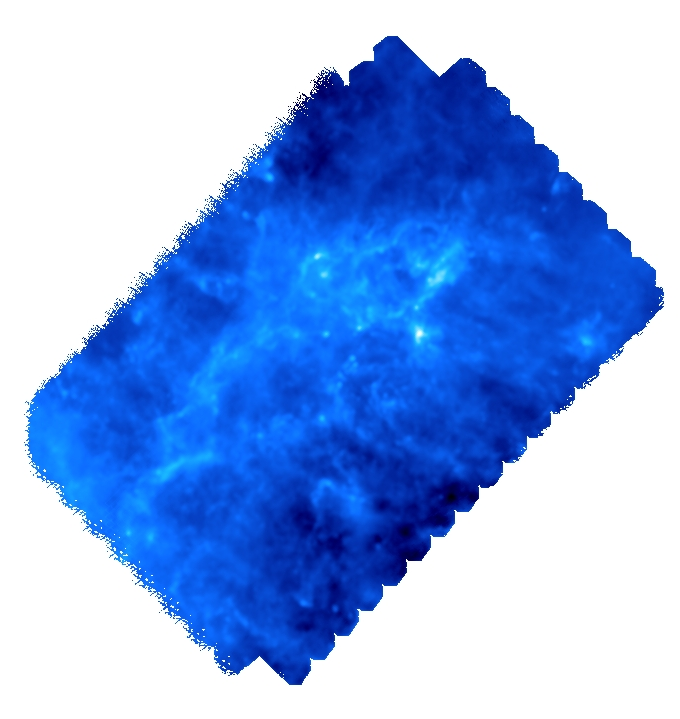
In this tutorial, we will identify the persistent filamentary structures in a diHydrogen column density map of the interstellar medium in the Eagle Nebula (M16) as observed by Herschel . The map is encoded in a 2D double precision FITS image, with pixels set to NaN in unobserved regions:
By default, mse will automatically mask NaN valued pixels so the FITS file could theoretically be fed directly to it. However, because of the complexity of the geometry of the observed region, it is preferable to use a mask to limit the analysis to a well defined region of interest (in particular, it is preferable that this region is simply connected - i.e. does not contain holes -). Designing a mask is relatively simple, as it consists in an image with pixels set to 0 in non-masked region and any other value in the masked regions (this behavior can be changed by adding a trailing '~' to the mask filename, see option -mask). The following mask was created with Gimp and saved as a .PNG file (any readable field file format is acceptable):
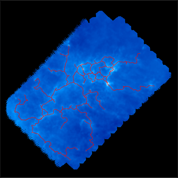
With this mask, we can now use mse to identify the filamentary structures in the map (option -upSkl) with the help of an interactive persitence diagram (option -interactive) to select the correct persistent threshold as we do not want to impose any à-priori on its value. We therefore run the following command:
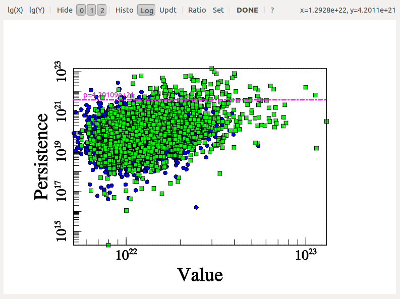
After some computations, the following diagram should appear (use buttons logX/logY to switch logarithmic coordinate and buttons 1, 2 and 3 to show/hide different types of persistence pairs):
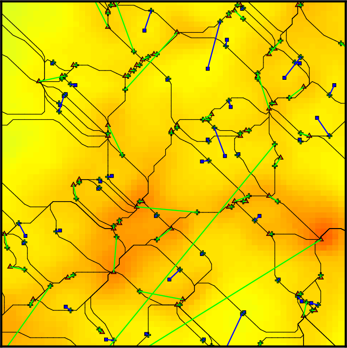
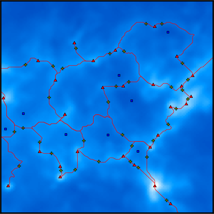
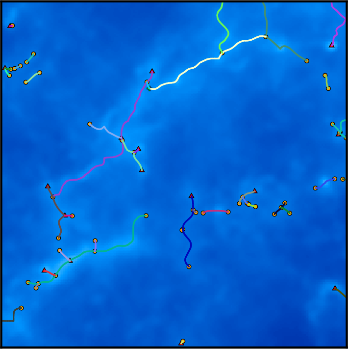
On this diagram, each dot represents a persistence pair of critical points (see overview section), with its X coordinate being the value at the lowest critical point of the two (i.e. the background density) and its Y coordinate the persitence of the pair (i.e. the value difference between the two, interpreted as contrast of the topological feature it represents with respect to its background). Points located in the right side of this diagram represent features located in high valued regions of the map, while points in the upper side represent features that clearly stand out from their background. More specifically, the green squares stand for pairs of type 1 (i.e. saddle-point / maximum pairs) while blue disks stand for pairs of type 0 (i.e. minimum saddle-point pairs). This can be easily visualized on the following image, which represents a zoom on the map with critical points identified as blue squares, green crosses and red triangles for minima, saddle points and maxima respectively. On this plot, the identified filaments are represented in black, and each persistence pair of type 0 or 1 is represented as a blue or green segment linking its two critical points together (each segment corresponds to one point in the persistence diagram above):
Basically, in 2D, removing a pair of type 0 (i.e. cancelling two critical points linked by a blue segment) amounts to deleting a piece of filament (i.e. 2 arcs departing from the saddle point) by merging two voids while removing a pair of type 1 (i.e. cancelling two critical points linked by a green segment) amounts to gluing pieces of filaments into longer ones (i.e. two arcs departing from the saddle point with one other arc departing from the maximum). When selecting the persistence threshold without à-priori, we therefore want to keep only the pairs that stand out of the general distribution on the Y-axis (i.e. with high persitence) so that only the most significant topological features remain. Selecting a threshold of ~4.2E21 as shown on the persistence diagram above seems quite reasonable (using Ctrl+left Click, and clicking on the DONE button to proceed).
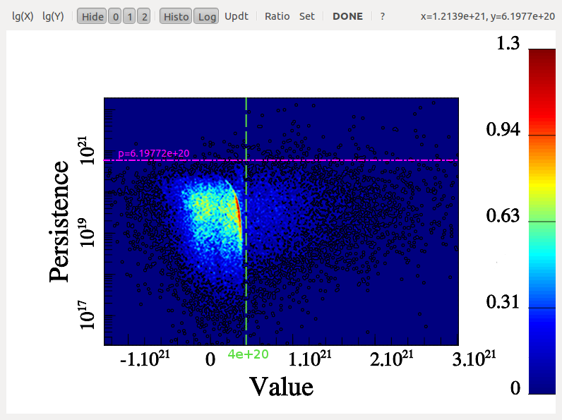
Visualizing a persistence diagram is a good way to determine the persistence threshold when assuming no previous knowledge of the data set. Note however that persistence could also have been set à-priori to the estimated amplitude of what is considered non-meaningful features or noise with option -cut <val> instead of -interactive. It is nonetheless always useful to check the persistence diagram as it deeply reflects the topological nature of the distribution and can be used to understand it better. For instance, the following diagram (represented by a 2D histogram of the pairs distribution, instead of the pairs themselves) was computed from a totally different map, and it is a good example:
Indeed, from this diagram, not only can one learn that the persistence threshold should be ~6.E20 (from the Y-axis), but one can easily see that the nature of the distribution is different for background values below or above "X=~4E20" on the X-axis. This feature reflects the fact that in some regions of this data-set, the signal was below the instrument detection threshold and the result is complex noise generated by the detectors. Meaningful features may stand out from these regions, so it does not affect the choice of the persistence threshold. However, this tells us that any region with a value <4E20 cannot be considered signal and identified filaments should therefore be trimmed wherever the value is below this threshold (this can be achieved by running mse with a persitencce threhold of 6.E20 and then running the following command on the output skeleton file: skelconv filaments.NDskl -trimBelow 4.E20).
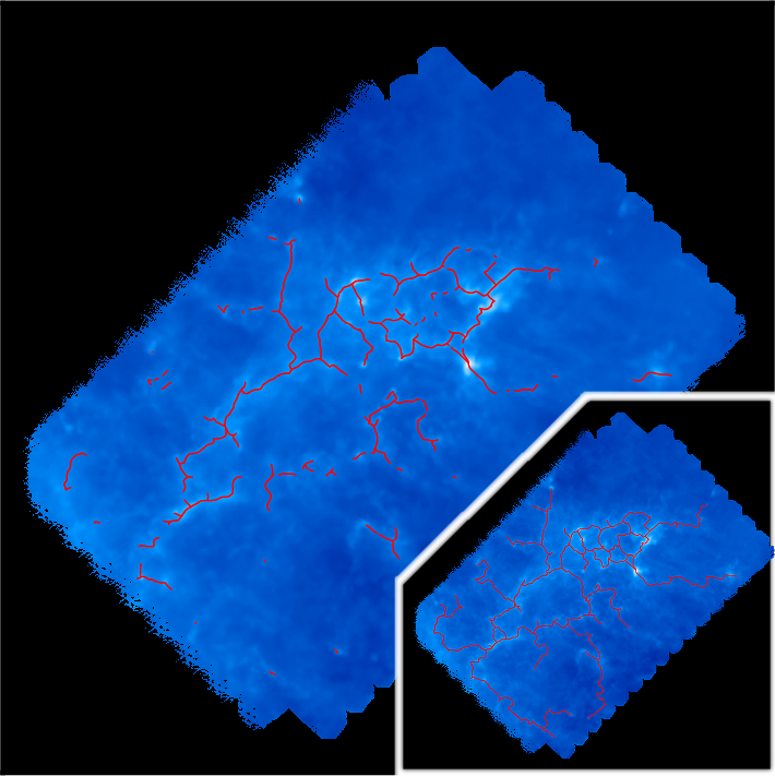
Let us now come back to our example, where no such trimming is necessary. Selecting a persistence threshold of ~4.2E21 as discussed previously, we obtain the following filamentary structures :
Remember that DisPerSE identifies structures as features of the Morse-Smale complex. The output of mse is always a valid (subset of the) Morse-Smale complex. In particular, filaments are identified as the set of arcs joining maxima and critical points, which means that pieces of filament always link a maximum and a critical point: they cannot stop in any other point, and whenever two filaments merge in points that are not maxima (i.e. bifurcation point), they remain distinct filaments until they reach a maximum (i.e. although they are not visually distinct as they are infinitely close, they are still stored as separate arcs in the output file). This is illustrated on the following figure, which shows a zoom on the identified filamentary structures with minima, saddle points and maxima represented as blue squares, green crosses and red triangles respectively:
On this figure, individual pieces of filaments (i.e. arcs) link red triangles to green crosses, and several pieces of arcs may therefore overlap above bifurcation points. This is of course desirable for mathematical applications that require the computation of valid Morse-Smale complexes but can be problematic when one only needs to identify structures and measure their properties. Indeed, regions where several arcs overlap may accidentally be given a stronger weight in statistical analysis, biasing the results. One can fix this with the option -breakdown of skelconv which is used to identify bifurcation points (adding them as dummy critical points of critical index D+1) and break filaments down into individual pieces of arcs.
Another problem is the resolution of the filaments, which is roughly equal to that of the underlying map: filaments are described as sets of small segments linking neighbor pixels together in the oupout files of mse. As a result, they appear jagged on the previous image and they can locally only take a discrete set of orientation. Using option -smooth N of skelconv, one can fix this by ensuring their smoothness over a size of ~N pixels. Note that only individual arcs or pieces of arcs are smoothed when using this option, critical points and bifurcation points remain fixed. As a result, the order of options -smooth and -breakdown on the command line is important.
We choose to first smooth over ~6 pixels and then break the network down :
The result is illustrated on the following figure:
where filaments are now smooth and bifurcation points are now identified as yellow discs : pieces of filament now link critical or bifurcation points and therefore do not overlap anymore.
Although the resulting filaments are perfectly usable as such for analysis, other useful post-treatment are available in DisPerSE. We give in the following an example of their possible usage, but note that it should of course be adapted to the particular results one wants to obtain ...
Options -trimAbove and -trimBelow for instance allow trimming portion of arcs so that they do not have to start/stop at critical or bifurcation points (dummy critical nodes are added at their extremities). By default, these options will trim the filaments above or below a given value of the field (see e.g. the example in the section on the persistence diagram above), but filaments can also be trimmed in any value tagged within the skeleton file (the list of the tags can be displayed by running skelconv filaments.NDskl -info and arbitrary tags can be added with option -addField).
A useful trimming function is robustness or robustness_ratio, which is not tagged by default in the skeleton files but can computed using option -robustness of mse (you can use option -loadMSC to avoid recomputing the whole Morse-Smale complex):
Robustness implements an improved version of the concept of separatrix persistence (Weinkauf, T. and Gunther, D., 2009) that allows the extension of regular persistence to each points of the filaments (as opposed to critical points pairs). Running the following command:
one can select the most meaningful subset of the filaments (you can try several robustness thresholds to see the result, but the selected threshold should probably be greater than the persistence threshold). Note that the concepts of persistence and robustness are different, and robustness basically allows selecting those subsets of persistent (topological) filaments that are most prominent. For that reason, it may make sense when trimming on robustness criteria to lower the persistence threshold (in mse) so that the significant pieces of less persistent filaments can still be conserved (you should probably experiment in order to find the best compromise between persistence and robustness thresholds for a given type of data set).
In the present case, choosing a robustness threshold of 8E21 (i.e. slightly higher than the persistence threshold), one obtains the following filaments:
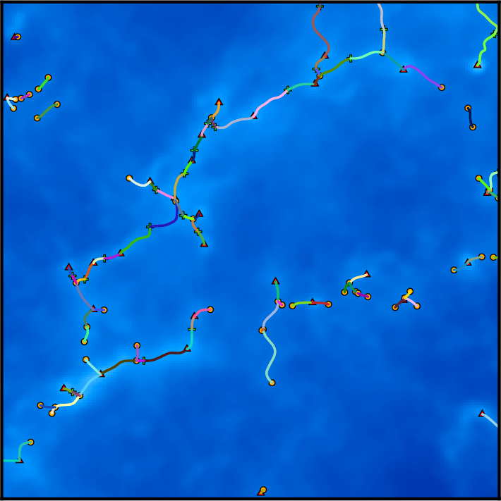
Another interesting post-treatment is the option -assemble that allows merging individual aligned pieces of filaments into larger structures. On the following picture, each piece of filament is represented with a distinct color:
Running the following command (note once again that the order of arguments is important, try changing it ...):
one can assemble pieces of filaments that form an angle smaller than 70 degrees, resulting in the following structures, where individual pieces are straight but as long as possible:
This tutorial uses file ${DISPERSE}/data/simu_2D.ND which contains the projected distribution of the particles in a slice of an N-Body dark matter simulation of a 50 Mpc large chunk of the universe. Note that although we use a 2D slice for convenience here, the following procedure would also work with the full 3D distribution.
In this example, the voids and filaments of the particle distribution will be computed from the underlying density function traced by the particles, so we first need to define the topology of the space (i.e. we need a notion of neighborhood for each particle) and to estimate the density function. This is achieved using the Delaunay tessellation of the particle distribution, which can be computed with delaunay_2D.
The distribution of the particles is periodic, so we could simply run:
delaunay_2D simu_2D.ND -periodic
However, in this example we are going to pretend that the distribution has boundaries, which will make visualization easier (if boundary conditions are periodic, a filament crossing a boundary reappears on the other side, causing visual artifacts). We nevertheless would like to use the fact that boundary conditions are indeed periodic to correctly estimate density on the boundaries, which can be achieved using option -btype:
delaunay_2D simu_2D.ND -btype periodic
The output file is named simu_2D.ND.NDnet by default, and it contains the Delauany tessellation as an unstructured network in NDnet format, as well as the density function estimated using DTFE at each vertex (i.e. the additional vertex data labeled field_value in the NDnet file). This file can be fed directly to mse, but we have to choose a persistence threshold first.
Because the input file is a Delaunay tessellation, persistence is expressed as a ratio (density has a close to lognormal PDF) and the persistence threshold as a number of sigmas representing the probability that a persistence pair with given persistence ratio happens in a pure random discrete Poisson distribution. It is usually safe in such case to select a threshold between 2-sigmas and 4-sigmas, and we could directly compute the filaments of the distribution with the following command (see mse for more info):
mse simu_2D.ND.NDnet -nsig 3 -upSkl
However, in this example, we will use a persistence diagram to decide the correct threshold (in case you do not have pdview, replace -interactive with -nsig 3 in the following commannd) and we would also like to identify the voids in the distribution (i.e. the ascending 3-manifolds originating from critical points of critical index 0; see option -dumpManifolds of mse):
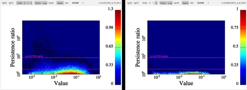
After running this command line, you should be able to visualize the following diagrams:
On this picture, the maxima/saddle persistence pairs diagram is represented on the left and the minima/saddle one on the right. The fact that the second type of pairs are clearly less persistent reflects the known fact that dark matter haloes are very prominent structures because they belong to regions in the non linear regime where density increases exponentially fast. One nice feature of persistence diagrams is that they make it easy to choose the threshold above which underlying topological structures stand out of the noise : in the present case, we want to select the high persistence tails only that clearly stand out from the bunch of pairs generated by noise. This gives us a threshold of around 3-sigmas that can be visually selected by clicking while holding Ctrl key down. Once the threshold is selected, simply press Done button.
After this operation, mse should output two files: the filaments in a skeleton type file (simu_2D.ND.NDnet_s3.up.NDskl) and the voids in a network type file (simu_2D.ND.NDnet_s3_manifolds_J0a.NDnet).
By default, mse associates maxima to vertices while minima are associated to d-simplices (where d is the dimension of space). As a result, the network representing the voids defines a set of triangles each associated to a given void. This may not be very practical for post-treatment or visualization, but we can use option -vertexAsMinima to reverse the convention (this will overwrite the previous file if the threshold is identical):
We can now visualize the result by converting the files to vtk formats using skelconv and netconv. The skeleton is smoothed and converted to vtp format:
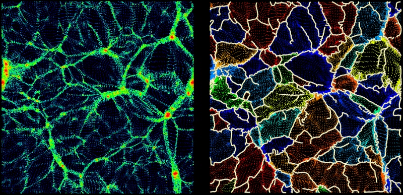
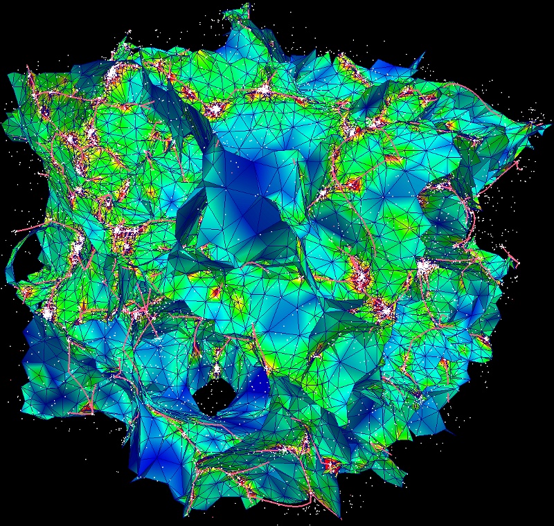
the result should look as follows when visualized with paraview: (the configuration file ${DISPERSE}/data/simu_2D_nonper.pvsm can be directly loaded in paraview (File->Load State) to produce the following plot)
Note: on the right figure, a different color is associated to the source_index of each particle depending on which void it belongs to: each void originates from a different minimum of the field and each critical point has a specific index. This source_index corresponds to the position of this critical point as a node in skeleton files or as a vertex in persistence pair networks obtained with mse (options -dumpArcs and -ppairs). It can therefore also be used to cross-link information contained in manifold networks and skeletons or persistence pairs, such as for instance retrieving the hierarchy of the voids (i.e. using the parent_index of the critical points in skeleton files and persistence pairs networks).
This tutorial follows the 2D discrete case example introduced in the previous section so you should probably read it first if you haven't done so yet.
We will compute the filaments and walls from the downsampled dark matter N-body simulation snapshot ${DISPERSE}/data/simu_32_id.gad. The distribution has periodic boundary conditions and we therefore start by computing its Delaunay tessellation with the following command:
delaunay_3D simu_32_id.gad -periodic
The program should output a file called simu_32_id.gad.NDnet that can be used directly with mse to compute the filaments and walls of the distribution. In 3D, walls are represented by the ascending 2-manifolds that originate from critical points of critical index 1 so they can be computed with option -dumpManifolds JE1a (letter E stands for Extended, which means that the ascending 1-manifolds and ascending 0-manifolds at the boundary of the walls will also be added, see option -dumpManifolds of mse) .Note that by default, subsets of the walls that are common to several walls are merged together, so you may want to try -dumpManifolds JP1a instead if you are interested in studying the properties of individual walls. The filaments are computed with option -upSkl or -dumparcs U which are equivalent. Using interactive mode to select a persistence threshold (use -nsig 3.5 instead of -interactive if pdview could not compile on your computer), we run the following command:
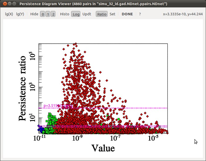
which after some quick computations, should display the following persistence diagram.
On this diagram, each type of pair is represented by a mark of different color : blue for minima/1-saddle, green for 1-saddle/2-saddle and red for 2-saddle/maxima. Note that the blue dots in the lower left corner stand for the voids in the distribution, so it is expected that we find only few of them compared to the red dots which represent collapsed structure (the simulation is 50 Mpc large). Each point on the diagram representing a topological feature, we would like to select only those points that stand out of the general distribution in terms of persistence in order to keep only the most meaningful structures (the persistence selection threshold is set by clicking while holding Ctrl key). The diagram suggests that persistence threshold should be above ~3-sigmas so we select a threshold of ~3.5 sigmas and click on the done button to confirm the selection. The program continues and should output the filaments in file simu_32_id.gad.NDnet_s3.52.up.NDskl and the walls in file simu_32_id.gad.NDnet_s3.52_manifolds_JE1a.NDnet.
It is instructive at that point to read mse output, and in particular the following section :
****** Simplifying complex ******
Starting Morse-Smale complex simplification.
Computing persistence pairs ... SKIPPED.
Sampling noise level was set to 3.5-sigma.
Cancelling pairs with persistance ratio < [2.66e+00,3.14e+00,4.42e+01].
   Tagging arcs ... done.
   Cancelling pairs (smart) ... (4140 rem.)
done.
   Cancellation took 0.10s (4140 canceled, 1 conflicts, 10 loops).
what mse tells us here is that it successfully removed 4140 persistence pairs, but was not able to cancel 11 more although their persistence was lower than the threshold. The 10 loops represent persistence pairs that were connected by more than one arc at the moment of their cancellation. Topologically speaking, their cancellation is not a valid operation as it would result in a discrete gradient loop (integral lines cannot form loops in Morse-theory). Note that the existence of non-cancellable pairs is not a bug of DisPerSE but rather a feature of Morse theory. However, not cancelling them may result in a few spurious non-significant pieces of filaments remaining in the ouput file (this is very problematic though as the impact on the identified filaments is very small in general) so one can use option -forceLoops to remove them anyway (which is perfectly fine if your goal is only to identify structures). Using this option will also solve the 1 conflict identified by mse, as conflicts are the result of a non-cancellable pair blocking the cancellation of a valid cancellable pair.
We can now rerun mse while skipping the computations by loading the backup file simu_32_id.gad.NDnet.MSC that mse generated on the previous run with option -loadMSC:
and visualize the result with paraview. The configuration file ${DISPERSE}/data/simu_32_per.pvsm can be directly loaded in paraview (File->Load State) to make the following plot: (note that it is a bit tricky to deal with periodic boundary conditions when visualizing, clipping the boundaries is usually the easiest way)
Note: contrary to the previous example where we computed 2D voids (see here), it is problematic in this case to identify each individual wall and paint it with a specific color. Indeed, contrary to voids, the 2-manifolds that represent walls can overlap, and so a unique source_index representing the critical point from which each wall originates cannot be assigned to each simplex (i.e. in that case, triangle). A solution to this problem would have been to specify that we wanted identical simplices to be stored as many times as they appear in different walls even though they are the same. This could have been achieved with flag P of option -dumpManifolds in mse:
As a result, the output file is larger, but it would also allow cross-linking the information contained in the geometry of the walls and that in the skeleton files or persistence pairs network (see this note).
This file type is designed to store the critical points and arcs of the Morse-Smale complex (i.e. one dimensionnal filamentary structures). In skeleton files, the filamentary network is described as lists of nodes representing critical points or bifurcation points if available (see option -breakdown of skelconv), lists of segments tracing the local geometry of arcs and filaments originating from and leading to nodes and described as lists of segments. The base skeleton format is NDskl which is used internally, but this format may be converted to several other more or less complex formats of skeleton files adapted to different applications (see option -to in program skelconv, a list of available formats is displayed when running the program without argument).
nb: Within skeleton files, the segments are always oriented in the ascending direction of the arcs, which does *NOT* necessarily mean that the value of the field is necessarily increasing locally ! Indeed, the value is locally allowed to fluctuate within the persistence threshold, so the field value does not have to be strictly increasing locally along an arc.
Available formats:
-NDskl (Read / Write): This is the format of the skeleton files created with mse. It is a relatively complex binary format that contains all the information on the geometry and connectivity of the arcs of the Morse-Smale complex (i.e. filaments).
-NDskl_ascii (Write only): This ASCII format contains the same amount of information as NDskl files, but organized in a different way. In particular, filaments are not described as lists of segments but rather each filament is described by an origin node, a destination node, and a set of sampling points.
-segs_ascii and crits_ascii (Write only): This is a simplified ASCII file format designed to be easily readable but that only contains a subset of the information available in NDskl files. In particular, segs_ascii files contain a list of individual segments describing the local orientation of the arcs as well as some limited information on the filament they belong to, while crits_ascii contain information on the critical points and bifurcation points only.
-vtk, vtk_ascii, vtp and vtp_ascii (Write only): These formats are binary and ASCII legacy and XML VTK formats that are readable by several 3D visualization tools, such as VisIt or ParaView for instance.
-NDnet (Write only): Using this format, skeleton files can be converted to unstructured networks (use netconv to convert NDnet files to other network formats).
Additional data: In addition to the topology and geometry of filamentary structures, more complete formats (i.e. NDskl, NDskl_ascii and all vtk formats) may store arbitrary additional information associated to filaments and nodes that can be used by skelconv (run skelconv filename.NDskl -info for a list of additional data available in skeleton file filename.NDskl). By default, mse stores the following additional data in skeleton type files:
-persistence / persistence_ratio / persistence_nsigmas (Nodes only) : The persistence (expressed as a difference, ratio or in number of sigmas) of the persistence pair containing the corresponding critical point. A negative or null value indicates that the node is not a critical point or that it does not belong to a persistence pair.
-persistence_pair (Nodes only): The index of the node that corresponds to the other critical point in the persistence pair (indices start at 0). The value is the index of the current node itself when it is not a critical point or it does not belong to a persistence pair.
-parent_index / parent_log_index (Nodes only): For each extrema only (i.e. minima and maxima), the index of the node that corresponds to the other extremum into which it would be merged if its persistence pair was canceled (indices start at 0). This can be used to reconstruct the tree of the hierarchy of maxima and minima. The value is -1 for non extrema critical points. The difference between the two versions is that the second (parent_log_index) is the hierarchy computed from the logarithm of the field. This second version is useful only for discrete point samples whose MS-complex is obtained from the delaunay tessellation computed with delaunay_nD. Practically, parent_log_index can be used whenever persistence pairs are cancelled in order of increasing ratio (option -nsig in mse), and parent_index whenever persistence pairs are cancelled in order of increasing difference (option -cut in mse).
-field_value / log_field_value (Nodes and Segments) : The value of the field and it logarithm. For segments, the suffix _p1 and _p2 is added to indicate which extremity of the segment it corresponds to.
-cell (Nodes and Segments) : The type and index of the cell corresponding to the node / segment in the initial network (i.e. from which the skeleton was computed). For segments, the suffix _p1 and _p2 is added to indicate which extremity of the segment it corresponds to. The value is a double precision floating number whose integer part is the index of the cell and decimal part its type. For instance, the 156th vertex (i.e. 0-cell) in the cell complex is represented as 156.0, while the 123th tetrahedron is 123.3. Note that the index of the 0-cell correpond to the index of the pixel / vertices in the original network from which the skeleton was computed.
-robustness / robustness_ratio (Nodes and Segments) : The robustness of the node / segment. Robustness is a local measure of how contrasted the critical point / filament is with respect to its local background, and it is therefore a good way to select only highly contrasted subsets of the filamentary structures (see option -trimBelow in skelconv). Note that robustness, like persistence, is defined as a difference or ratio between the value of the field in two points, so the robustness threshold has the same order of magnitude as the persistence threshold.
- type (Segments only) : The type of arc the segment belongs to. The value corresponds to the lowest critical index of the two critical points at the extremities of the arc the segments belongs to. For instance, in dimension D, the ridges (filaments) have type D-1.
This is the native binary format of DisPerSE. Functions for reading and writing NDskl format in C can be found within the file ${DISPERSE_SRC}/src/C/NDskeleton.c (see functions Load_NDskel, Save_NDskel and also Create_NDskel). In this format, the arcs of the Morse-Smale complex are described as arrays of nodes and segments with data associated to each of them. Each node contains information on critical points (which may also be bifurcations points or trimmed extremities of filaments). Each segment contains information on the local geometry of the arcs and global properties of the skeleton.
When using the C functions from Disperse, data is loaded into the following C structure which is close to the actual structure of the file (see file ${DISPERSE_SRC}/src/C/NDskeleton.h):
struct NDskl_seg_str {
   int nodes[2];  // index of the nodes at the extremity of the arc. Segment is oriented from nodes[0] toward nodes[1]
   float *pos;  // points to appropriate location in segpos
   int flags;  // non null if on boundary
   int index;  // index of the segment in the Seg array
   double *data;  // points to the nsegdata supplementary data for this segment
   struct NDskl_seg_str *Next; // points to next segment in the arc, NULL if extremity (->connects to nodes[1])
   struct NDskl_seg_str *Prev; // points to previous segment in the arc, NULL if extremity (->connects to nodes[0])
 };
 typedef struct NDskl_seg_str NDskl_seg;
 struct NDskl_node_str {
   float *pos;  // points to appropriate location in nodepos
   int flags;  // non null if on boundary
   int nnext;  // number of arcs connected
   int type;  // critical index
   int index;  // index of the node in the Node array
   int *nsegs; // number pf segments in each of the the nnext arcs
   double *data;   // points to the nnodedata supplementary data for this segment
   struct NDskl_node_str **Next;  // points to the node at the other extremity of each of the nnext arcs
   struct NDskl_seg_str **Seg;   // points to the first segment in the arcs, starting from current node.
 };
 typedef struct NDskl_node_str NDskl_node;
 typedef struct NDskel_str {
   char comment[80];

   int ndims;  // number of dimensions
   int *dims;  // dimension of the underlying grid, only meaningfull when computed from a regular grid
   double *x0;  // origin of the bounding box
   double *delta;  // dimension of the bounding box

   int nsegs;  // number of segments
   int nnodes;  // number of nodes

   int nsegdata;  // number of additional data for segments
   int nnodedata;  // number of additional data for nodes
   char **segdata_info;  // name of additional fields for segments
   char **nodedata_info;  // name of additional fields for nodes

   float *segpos;  // positions of the extremities of segments (2xndims coords for each segment)
   float *nodepos; // positions of the nodes (ndims coords for each segment)
   double *segdata; // additional data for segments (nsegs times nsegdata consecutive values)
   double *nodedata; // additional data for nodes (nnodes times nnodedata consecutive values)

   NDskl_seg *Seg;  // segment array (contains all segs)
   NDskl_node *Node;  // nodes array (contains all nodes)
 } NDskel;
The NDskl binary format is organized as follows (blocks are delimited by dummy variables indicating the size of the blocks for FORTRAN compatibility, but they are ignored in C):
NDskl binary format
field
type
size
comment
dummy
int(4B)
1
for FORTRAN compatibility
tag
char(1B)
16
identifies the file type. Value : "NDSKEL"
dummy
int(4B)
1
dummy
int(4B)
1
comment
char(1B)
80
a comment on the file (string)
ndims
int(4B)
1
number of dimensions
dims
int(4B)
20
dimension of underlying grid (0=none, ndims values are read)
x0
double(8B)
20
origin of bounding box (ndims first values are meaningful)
delta
double(8B)
20
size of bounding box (ndims first values are meaningful)
nsegs
int(4B)
1
number of segments
nnodes
int(4B)
1
number of nodes
nsegdata
int(4B)
1
number of additional data associated to segments.
nnodedata
int(4B)
1
number of additional data associated to nodes.
dummy
int(4B)
1
dummy
int(4B)
1
this block is ommited if nsegdata=0
seg_data_info
char(1B)
20×nsegdata
name of the segment data field
dummy
int(4B)
1
this block is ommited if nsegdata=0
dummy
int(4B)
1
this block is ommited if nnodedata=0
node_data_info
char(1B)
20×nnodedata
name of the node data field
dummy
int(4B)
1
this block is ommited if nnodedata=0
dummy
int(4B)
1
segpos
float(4B)
2×nsegs×ndims
coordinates of segment extremities
dummy
int(4B)
1
dummy
int(4B)
1
nodepos
float(4B)
nnodes×ndims
coordinates of nodes
dummy
int(4B)
1
dummy
int(4B)
1
segdata
double(8B)
nsegdata×nsegs
value of the segments data fields
dummy
int(4B)
1
dummy
int(4B)
1
nodedata
double(8B)
nnodedata×nnodes
value of the nodes data fields
dummy
int(4B)
1
dummy
int(4B)
1
following block is repeated for each node (×nnodes).
pos_index
int(4B)
1
index in the nodepos/nodedata arrays
flags
int(4B)
1
flags (identify boundary nodes)
nnext
int(4B)
1
number of connected arcs
type
int(4B)
1
critical index (ndims+1 for bifurcations / trimmed arc axtremity)
index
int(4B)
1
index of this node
nsegs
int(4B)
nnext
number of segments in each connected arc
*
*
*
blue section repeated for each connected arc (×nnext)
nextNode
int(4B)
1
index of the other node of the arc
nextSeg
int(4B)
1
index of the first segment on the arc
dummy
int(4B)
1
dummy
int(4B)
1
following block is repeated for each segment (×nsegs).
pos_index
int(4B)
1
index in the segpos/segdata arrays
nodes
int(4B)
2
index of the 2 nodes at the endpoints of the current arc.
flags
int(4B)
1
flags (identify boundary nodes)
index
int(4B)
1
index of this segment
next_seg
int(4B)
1
index of the next segment in the node (-1 if none)
prev_seg
int(4B)
1
index of the previous segment in the node (-1 if none)
An ASCII format that contains the same amount of information as NDskl files, but organized in a different way. In particular, filaments are not described as lists of segments but rather each filament is described by an origin node, a destination node, and a set of sampling points.
NDskl_ascii format
ANDSKEL
header
ndims
the number of dimensions
#comments go here
OPTIONAL: should start with '#' if present (the 80 first characters are read and stored).
BBOX [x0_1 .. x0_d] [delta_1 .. delta_d]
OPTIONAL: the bounding box, defined by the 'ndims' coordinates of the origin 'x0' and extent 'delta'.
[CRITICAL POINTS]
Marks the beginning of the critical points section
ncrit
The number of critical points (CP)
type pos[0] ... pos[ndims-1] value pairID boundary
Info on the first CP: critical index, position, value, index of CP in the persistence pair, 0 if not on the boundary
nfil
The number of filaments connected to this CP
destId[0] filId[0]
Info on the first filament: index of the CP at the other extremity of the filament, and index of the filament (see filaments table below)
...
One line for each filament connecting on the CP
destId[nfil-1] filId[nfil-1]
Information on the last filament
.....
.....
one blue block for each CP.
.....
[FILAMENTS]
Marks the beginning of the filaments section
nfil
Total number of filaments
CP1 CP2 nSamp
index of the CP at the extremity of the first filament and number of sampling points
P[0][0] ... P[0][ndims-1]
position of the first sampling point of first filament.
...
One line for each sampling point of first filament.
P[nSamp-1][0] ... P[nSamp-1][ndims-1]
Position of the last sampling point
.....
.....
one blue block for each filament.
.....
[CRITICAL POINTS DATA]
Marks the beginning of the CP data section
NF
Number of fields associated to each CP.
CP_DATA_FIELD_NAME_1
Name of the first field
...
CP_DATA_FIELD_NAME_NF
Name of the last field
val_1[0] ... val_NF[0]
Value of each field for first CP
...
val_1[N_CP-1] ... val_NF[N_CP-1]
Value of each field for last CP
[FILAMENTS DATA]
Marks the beginning of the filaments data section
NF
Number of fields associated to each sampling point of each filament.
FIL_DATA_FIELD_NAME_1
Name of the first field
...
FIL_DATA_FIELD_NAME_NF
Name of the last field
val_1[0][0] ... val_NF[0][0]
field values for first sampling point, first filament
...
val_1[0][nSamp[0]] ... val_NF[0][nSamp[0]]
field values for last sampling point, first filament
This ASCII format is a very simple one. It consists in a list of individual segments describing the local orientation of the arcs as well as some limited information on the filament they belong. This may be used for doing statistical analysis of local properties of filaments such as the local orientation of a magnetic field for instance. Note that all the segments are oriented from the lower critical index extremity of the filament they belong toward the other extremity (which does NOT mean that the value is strictly increasing, as local fluctuations of amplitude the persistence threshold are still allowed ... ).
nb: you probably want to use option -breakdown of skelconv before using this format.
segs_ascii format
#arc segments
Header
#U0 U1 U2 V0 V1 V2 value_U value_V type boundary
Header identifying each column
#NDIMS NSEGS
Number of dimensions and number of segments
U0 U1 U2 V0 V1 V2 value_U value_V type boundary
The value of the fields for the first segment
....
One such line for each NSEGS segment
Notations:
-U_0,..., U_ndims : The coordinates of the first extremity of the segment. It is the one closest to the lowest critical index CP along the filament it belongs to.
-V_0,..., V_ndims : The coordinates of the second extremity of the segment. It is the one closest to the highest critical index CP along the filament it belongs to.
-value_U, value_V : Value of the field in U and V.
-type : the type of arc the segment belongs to. The type of an arc is the minimum critical index of the CP at the extremity of the filament the segment belong to.
-boundary : value can be 0, 1 or 2 when the segment is inside the domain, on the boundary, or outside (e.g. at infinity)
This ASCII format is a very simple one. It consists in a list of all the critical points with some useful information for each of them.
crits_ascii format
#critical points
Header
#X0 X1 X2 value type pair_id boundary
Header identifying each column
#NDIMS NPOINTS
Number of dimensions and number of points
X0 X1 X2 value type pair_id boundary
The value of the fields for the first point
....
One such line for each NPOINTS points
Notations:
-X_0,..., X_ndims : the coordinates of the pooint
-value : Value of the field.
-type : the critical index of the point. A value of NDIMS+1 indicates a bifurcation point or a trimmed extremity.
-pair_id : index of the other critical point in the persistence pair. C style convention is used, indices starting at 0, and points without perisstence pairs have their own index for pair_id.
-boundary : value can be 0, 1 or 2 when the point is inside the domain, on the boundary, or outside (e.g. at infinity)
VTK formats are developed for the Visualization Tool Kit library (VTK) and can be used for 3D visualization with software such as VisIt or ParaView. Skeletons are stored as VTK polygon data and can be output in fours different VTK formats:
-vtk: the legacy format
-vtk_ascii: ASCII version of the vtk format
-vtp: a more recently developed XML version of the vtk format,
-vtp_ascii: ASCII version of the vtp format
The specifications for these formats can be found in this PDF file. See also here and there for additional information.
This file type is designed to store any kind of unstructured network (such as delaunay tesselations or more generally cell complexes). In DisPerSE, its usage is restricted to networks of simplices though, and it is mainly used to store ascending and descending manifolds (voids and walls for instance) and persistence pairs as output by mse or Delaunay tessellations as output by delaunay_nD (skeleton files can also be converted to networks using skelconv -to NDnet). Within network files, networks are represented by setz of vertices and cells of any dimension. A n-cell is a cell of dimension n, which is therefore described, in the case of a simplicial network, as a set of n+1 vertices index. In the case of a simplicial complex, only the highest dimensional cell have to be explicitly given, but other type of cells may also be specified. Indeed, extended manifolds for instance are not described as complexes: an ascending 0-manifold in 3D is a set of tetrahedrons (3-cells), triangles (representing ascending 1-manifolds on its boundary), segments (ascending 2-manifolds on its boundary) and vertices (ascending 3-manifolds / critical points). Note that additional information can also be associated to each type of cell (see below).
The base network format is NDnet which is used internally, but this format may be converted to several other more or less complex formats of network files adapted to different applications (see option -to in program netconv, a list of available formats is displayed when running the program without argument).
Available formats:
-NDnet (Read / Write): This is the format of the network files created or red by mse. It is a relatively complex binary format (it is actually more complex than needed as it is designed to store generic non-simplicial networks) that contains all the information on the geometry and topology of unstructured networks as well as additional data associated to each type of cells.
-NDnet_ascii (Read / Write): This ASCII format contains the same amount of information as NDnet files, but restricted to simplicial networks. It is easy to read and write so it may be used to write reasonably sized networks used as input for mse.
-PLY and PLY_ascii (Read binary only / Write): This is a rather popular and simple binary or ASCII format that can be used as an interface with other software.
-vtk, vtk_ascii, vtu and vtu_ascii (Write only): These formats are binary and ASCII legacy and XML VTK formats that are readable by several 3D visualization tools, such as VisIt or ParaView for instance.
Additional data: In addition to the topology and geometry of the network, arbitrary additional information may be associated to each type of cell. Run netconv filename -info for a list of additional data available in the network file filename. By default, the name of additional data added by mse is relatively explicit, it includes (see also the additional data section of the skeleton file format description):
-field_value / log_field_value : The value of the field and its logarithm. The tag field_value corresponds to the input function for mse, whose Morse-Smale complex is to be computed.
-cell: The type and index of a cell in the original network (prefix may be added). The value is a double precision floating number whose integer part is the index of the cell and decimal part its type. For instance, the 156th vertex (i.e. 0-cell) in the cell complex is represented as 156.0, while the 123th tetrahedron is 123.3. Note that the index of the 0-cell correpond to the index of the pixel / vertices in the original network from which the skeleton was computed.
-type: This usually corresponds to the critical index of a critical point (for instance, vertices of persistence pairs networks), or the type of a persistence pair (i.e. the minimum critical index of the CP in the pair, for segments of persistence pairs networks).
-index Usually the index of a vertex (e.g. for persistence pairs, additional segment data tagged up_index and down_index correspond to the indices of the vertices with lowest and highest critical index in the persistence pair respectively).
-persistence / persistence_ratio / persistence_nsigmas : The persistence (expressed as a difference, ratio or in number of sigmas) of the persistence pair containing the corresponding critical point. A negative or null value indicates that persistence is not relevant to this particular cell.
-parent_index / parent_log_index (vertices only): For persistence pairs type networks, for each vertex representing an extremum (i.e. minima and maxima), the index of the vertex that corresponds to the other extremum into which it would be merged if its persistence pair was canceled (indices start at 0). This can be used to reconstruct the tree of the hierarchy of maxima and minima. The value is -1 for non extrema critical points. The difference between the two versions is that the second (parent_log_index) is the hierarchy computed from the logarithm of the field. The second version is useful only for discrete point samples whose MS-complex is obtained from the delaunay tessellation computed with delaunay_nD. Practically, parent_log_index can be used whenever persistence pairs are cancelled in order of increasing ratio (option -nsig in mse), and parent_index whenever persistence pairs are cancelled in order of increasing difference (option -cut in mse).
-source_cell / source_index: For networks representing manifolds (voids, walls, ... obtained with option -dumpManifolds of mse), this represents for each simplex the critical point from which the manifold it belongs to originates (for instance, the minimum corresponding to a void, or the saddle point corresponding to a filament). In source_cell, the critical points is represented by its cell in the initial cell complex (see cell above), while source_index gives the index of the critical point in the skeleton file or persistence pair network obtained with mse (options -dumpArcs and -ppairs). See also here and there in the tutorial section.
This is the native binary format of DisPerSE. Functions for reading and writing NDnet format in C can be found within the file ${DISPERSE_SRC}/src/C/NDnetwork.c (see functions Load_NDnetwork and Save_NDnetwork). The format may seem relatively complex, but most of it is actually optional and not used in disperse (only simplicial complexes are used in DisPerSE). To create DisPerSE input files, it is only necessary to define the highest dimensional n-simplices as a list of (n+1) vertices (see also function CreateNetwork).
Note: The scalar function whose MS-complex is computed by mse can be stored as an additional data field
named 'field_value' (case sensitive).
Warning: in the following, for legacy reasons, the terms n-face and n-cell are used indifferently to designate polygons of dimension n (which are always simplexes in DisPerSE).
When using the C functions from Disperse, data is loaded into the following C structure which is close to the actual structure of the file (see file ${DISPERSE_SRC}/src/C/NDnetwork.h):
typedef struct
 {
   int type; // the cell-type
   char name[255];  // name of the field
   double *data;  // value for each of the nfaces[n] n-cells
} NDnetwork_Data;
// NDnetwork_SupData is not used in disperse ...
typedef struct
{
   int type;
   char name[255];
   int datasize;
   char datatype[255];// a string to identity how data should be casted
   void *data;
} NDnetwork_SupData;
typedef struct
{
   char comment[80];
   int periodicity;
   int ndims; // the number of spatial dimensions
   int ndims_net; // number of dimension of the network itself (e.g. 2 for a sphere embedded in 3D)
   int isSimpComplex;  // 1 if network is a simplicial complex (always true in disperse)
   double *x0;  // origin of the bounding box
   double *delta;  // size of the bounding box
   int indexSize; // size of NDNET_UINT type in Bytes
   int cumIndexSize; // size of NDNET_IDCUMT type in Bytes
   char dummy[160-4*2]; // dummy data reserved for future extensions

   NDNET_UINT nvertex;  // total number of vertices
   float *v_coord; //vertices coodinates (X_0,Y_0,Z_0,X_1,Y_1,...,Z_nvertex-1)

   NDNET_UINT *nfaces; // number of cells of a given type t is given by nfaces[t]

   int *haveVertexFromFace; // haveVertexFromFace[n] is 1 if we have an explicit definition of the n-cells (at least one type of cell must be defined).
   NDNET_IDCUMT **f_numVertexIndexCum;// cumulative number of vertice in the t-cells, NULL when cells are simplexes (isSimpComplex=1)
   NDNET_UINT **f_vertexIndex; // list of vertices defining the n-cells is stored in f_vertexIndex[n], all vertices being enumerated for each cell (the indices of the vertices in the kth n-cell start at f_vertexIndex[n][(n+1)*k] )
   // see also macro  NUM_VERTEX_IN_FACE(net,type,face) and VERTEX_IN_FACE(net,type,face)

   //This may be computed internally within DisPerSE but does not need to be defined explicitely
   int *haveFaceFromVertex; // haveFaceFromVertex[n] is 1 if we have an explicit list of all the n-cells that contain each vertex (used to navigate within the network)
   NDNET_IDCUMT **v_numFaceIndexCum; // cumulative number of t-cells a vertex v belongs to
   NDNET_UINT **v_faceIndex; // indices of the t-cells in the co-boundary of v ( the list of n-cells of vertex k starts at v_faceIndex[n][net->v_numFaceIndexCum[n][k]] and ends at v_faceIndex[n][net->v_numFaceIndexCum[n][k+1]] )
   // see also macro  NUM_FACE_IN_VERTEX(net,type,vertex) and  FACE_IN_VERTEX(net,type,vertex)

   // This can become extremely memory heavy ... NOT used in DisPerSE
   int **haveFaceFromFace; // haveFaceFromFace[k][n] is 1 if we have an explicit list of all the n-cells that have a boundary/co-boundary relation with each k-cell (used to navigate within the network)
   NDNET_IDCUMT ***f_numFaceIndexCum; //  cumulative number of n-cells having a boundary / co-boundary relation with each k-cell: f_numFaceIndexCum[k][n]
   NDNET_UINT ***f_faceIndex; // indices of the cells (similar to v_faceIndex)
   // see also macro NUM_FACE_IN_FACE(net,ref_type,ref_face,type) and FACE_IN_FACE(net,ref_type,ref_face,type)

   int haveVFlags;  // do we have flags associated to each vertex ?
   int *haveFFlags;  // do we have flags associated to each n-cell ?
   unsigned char *v_flag; // nvertex flag values (1 for each vertex) or NULL
   unsigned char **f_flag; // nfaces[n] flag values (1 of each n-cell) or NULL

   int ndata; // number of additional data fields.
   NDnetwork_Data *data; // array of all additionnal data (data in total)

   int nsupData;
   NDnetwork_SupData *supData;

} NDnetwork;
The NDnet binary format is organized as follows (blocks are delimited by dummy variables indicating the size of the blocks for FORTRAN compatibility, but they are ignored in C):
NDnet binary format
field
type
size
comment
dummy
int(4B)
1
for FORTRAN compatibility
tag
char(1B)
16
identifies the file type. Value : "NDNETWORK"
dummy
int(4B)
1
dummy
int(4B)
1
ndims
int(4B)
1
number of dimensions of the embedding space
ndims_net
int(4B)
1
ndims spanned by the network (=ndims by default)
dummy
int(4B)
1
dummy
int(4B)
1
comment
char(1B)
80
a comment on the file (string)
periodicity
int(4B)
1
0=non periodic, if p^th bit is set, boundary are periodic along dimension p
isSimpComplex
int(4B)
1
1 if network is made of simplices (must be 1 for DisPerSE)
x0
double(8B)
ndims
origin of bounding box
delta
double(8B)
ndims
size of bounding box
index_size
int(4B)
1
size of NDNET_UINT integer format in Bytes
cumindex_size
int(4B)
1
size of NDNET_IDCUMT integer format in Bytes
dummy_ext
char(1B)
152
dummy data reserved for future extensions
nvertex
NDNET_UINT
1
number of vertices
dummy
int(4B)
1
dummy
int(4B)
1
v_coords
float(4B)
ndims×nvertex
coordinates of the vertices [X0,Y0, ...]
dummy
int(4B)
1
dummy
int(4B)
1
nfaces
NDNET_UINT
ndims+1
number of cells of each type (N0,N1,...)
dummy
int(4B)
1
dummy
int(4B)
1
haveVertexFromFace
int(4B)
ndims+1
are n-cells explicitly defined ? (0=no, 1=yes)
dummy
int(4B)
1
*
*
*
next 3 lines are repeated for each (ndims+1) possible cells type , only if haveVertexFromFace[n] is true.
dummy
int(4B)
1
f_vertexIndex[n]
NDNET_UINT
(n+1)×nfaces[n]
list of (n+1) vertex indices for each n-cell
dummy
int(4B)
1
dummy
int(4B)
1
haveFaceFromVertex
int(4B)
ndims+1
are n-cells in the co-boundary of each vertex explicitly defined ? (0=no, 1=yes)
dummy
int(4B)
1
*
*
*
next 6 lines are repeated for each (ndims+1) possible cells type, only if haveFaceFromVertex[n] is true.
dummy
int(4B)
1
numFaceIndexCum[n]
NDNET_IDCUMT
nvertex+1
cumulative count of n-cells on vertices co-boundary
dummy
int(4B)
1
dummy
int(4B)
1
v_faceIndex[n]
NDNET_UINT
numFaceIndexCum[n]
list of n-cells on the co-boundary of each vertex (vertex i have numFaceIndexCum[n][i+1]-numFaceIndexCum[n][i] of them)
dummy
int(4B)
1
dummy
int(4B)
1
haveFaceFromFace
int(4B)
(ndims+1)^2
are n-cells in the co-boundary of each k-cell explicitly defined ? (0=no, 1=yes)
dummy
int(4B)
1
*
*
*
This section describes boundary relation between n-cells and k-cells. It is usually empty in DisPerSE (see NDnetwork.c for details) so SKIP IT :)
dummy
int(4B)
1
haveVFlags
int(4B)
1
1 if vertex flags are defined
dummy
int(4B)
1
*
*
*
next 3 lines are skipped if haveVFlags=0
dummy
int(4B)
1
v_flag
uchar(1B)
nvertex
value of the flags for vertices
dummy
int(4B)
1
dummy
int(4B)
1
haveFFlags
int(4B)
ndims+1
1 if flags are defined for n-cells
dummy
int(4B)
1
*
*
*
next 3 lines are repeated for each n-cell such that haveFFlags[n]=1
dummy
int(4B)
1
f_flag[n]
uchar(1B)
nfaces[n]
value of the flags for n-cells
dummy
int(4B)
1
dummy
int(4B)
1
ndata
int(4B)
1
total number of additional fields
dummy
int(4B)
1
*
*
*
next 7 lines are repeated for each additional field (×ndata)
dummy
int(4B)
1
type
int(4B)
1
the type of cells (0=vertex, n = n-simplex)
name
char(1B)
255
name of the supplementary data
dummy
int(4B)
1
dummy
int(4B)
1
data
double(8B)
N
data associated to cells or vertices. N is nfaces[n] or nvertex depending on the type value.
This ASCII format is a simpler version of the NDnet format, designed to be fully compatible but restricted to simplicial networks. It is easy to read and write and should probably be used for reasonably sized data sets.
Note: The scalar function whose MS-complex is computed by mse can be stored as an additional data field
named 'field_value' (case sensitive).
NDnet_ascii format
ANDNET
header
ndims
the number of dimensions
#comments go here
OPTIONAL: should start with '#' if present (the 80 first characters are read and stored).
BBOX [x0_1 .. x0_d] [delta_1 .. delta_d]
OPTIONAL: the bounding box, defined by the 'ndims' coordinates of the origin 'x0' and extent 'delta'.
nv
number of vertices
vx[0] vy[0] ...
the ndims coordinates of the first vertex
...
One line for each vertex
Simplices definition (0-cells up to ndims-cells). One blue block should be added for each type of explicitly defined simplex. Note that only the highest dimension cells are sufficient to define a complex.
T N
network has N T-simplices (each T-simplex has (T+1) vertices).
i[0] j[0] ...
the T+1 indices (start at 0) of the vertices of the first T-simplex.
...
one line for each of the N T-simplices
[ADDITIONAL_DATA]
OPTIONAL: indicate the beginning of the additional data section
additional_data_name_1
name of the additional data (e.g. field_value for mse input files)
T
type of simplex it is associated to (T-simplex, 0 means vertices)
The PLY format is a relatively generic file format designed to store three dimensional data from 3D scanners with the possibility of associating properties to the polygons. Information on this format can be found on wikipedia (see also the External links section). A very efficient C library for reading and writing PLY files in ASCII or binary format is RPly (DisPerSE uses it for PLY files I/O, see files NDnet_PLY_IO.c and NDnet_PLY_IO.h).
A typical header for a PLY file readable by netconv or mse is as follows:
ply
format ascii 1.0
element bbox 1
property list uchar double x0
property list uchar double delta
element vertex 77595
property float x
property float y
property float z
property double field_value
element face 482867
property list uchar uint vertex_indices
end_header
-format may be ASCII or little / big endian binary
-bbox element is used to define a bounding box if available (x0 is its origin and delta its extent)
-coordinates of the vertices are given as vertex properties labeled x, y, and z or x0, x1, ... (the number of this properties gives the dimension of the embedding space)
-faces are defined by the property vertex_indices, each element corresponding to a list of vertices. A cell is always supposed to be a simplex, so the number of vertices determine the dimension spanned by the complex (a 2D complex may be embedded in a 3D space).
-additional properties may be defined for cells and vertices. In particular, a vertex property labeled field_value would be used as input function in mse.
VTK formats are developed for the Visualization Tool Kit library (VTK) and can be used for 3D visualization with software such as VisIt or ParaView. Networks are stored as VTK unstructured network data and can be output in fours different VTK formats:
-vtk: the legacy format
-vtk_ascii: ASCII version of the vtk format
-vtu: a more recently developed XML version of the vtk format,
-vtu_ascii: ASCII version of the vtu format
The specifications for these formats can be found in this PDF file. See also here and there for additional information.
This file type is designed to store scalar fields sampled over regular grids (i.e. regular images in 2D, 3D and more) or, by extension, coordinates of tracer particles sampling an underlying density field. The main field format is NDfield, which allows to store any type of data (integer, simple or double precision floating point, ...) over arbitrary sized regular grids or as coordinates of tracer particles.
Available formats:
-NDfield (Read / Write): This is the format used internally in DisPerSE, it is efficient and generic as it can store regular grids or sample particles coordinates indifferently.
-NDfield_ascii (Read / Write): A simple ASCII version of the NDfield format, it is as versatile but data is always considered to be double precision floating point.
-FITS (Read only): Used to read 2D or 3D regular grids of arbitrary dimensions in the popular Flexible Image Transport System (FITS) image format. Also used for HEALPIX tessellations of the sphere.
-survey_ascii(Read only): A simple ASCII format whose main purpose is to easily read coordinates of discretely sampled astrophysical surveys (e.g. such as an SDSS galaxy catalog). Try this if you use spherical coordinates or if distance is measured by redshift for instance.
-SDL-image (Read only): This input format is used to read 2D regular grids encoded in a popular picture format readable by SDL-image library (jpg, png, gif, ...).
-vtk, vtk_ascii, vti and vti_ascii (Write only): These formats are binary and ASCII legacy and XML VTK formats that are readable by several 3D visualization tools, such as VisIt or ParaView for instance.
-NDnet (Write only): Using this format, field files representing tracer particles coordinates can be converted to unstructured networks (use netconv to convert NDnet files to other network formats). Regular grids conversion is not implemented yet due to the huge size of the output network.
This is the native binary format of DisPerSE. Functions for reading and writing NDfield format in C can be found within the file ${DISPERSE_SRC}/src/C/NDfield.c (see functions Load_NDfield and Save_NDfield).
When using the C functions from Disperse, data is loaded into the following C structure which is close to the actual structure of the file (see file ${DISPERSE_SRC}/src/C/NDfield.h):
typedef struct NDfield_str
{
 char comment[80];  // a comment on the data
 int dims[NDFIELD_MAX_DIMS];  // dimensions of the grid, must be [ndims,nparticles] when data represents sample particles coordinates (i.e. when fdims_index!=0)
 int ndims;  // number of dimensions of the space
 int n_dims;  // number of meaningfull values in dims array
 int fdims_index; // if 0, the field is a regular grid of dimensions dims, else the file contains the dims[0] coordinates of dims[1] particles.
 int datatype;  // type of the data (one of the ND_... defined above)
 double x0[NDFIELD_MAX_DIMS];  // origin of the bounding box
 double delta[NDFIELD_MAX_DIMS];  // extent of the bounding box
 char dummy[160];  // dummy data, for future extensions or for storing anything you want.

 void *val;  // pointer to data

 long nval;  // total number of particles (fdims_index==1) or pixels (fdims_index==0)
 int datasize;  // size in bytes of datatype type.
} NDfield;
The NDfield binary format is organized as follows (blocks are delimited by dummy variables indicating the size of the blocks for FORTRAN compatibility, but they are ignored in C):
NDnet binary format
field
type
size
comment
dummy
int(4B)
1
for FORTRAN compatibility
tag
char(1B)
16
identifies the file type. Value : "NDFIELD"
dummy
int(4B)
1
dummy
int(4B)
1
ndims
int(4B)
1
number of dimensions of the embedding space
dims
int(4B)
20
size of the grid in pixels along each dimension, or [ndims,nparticles] if data represents particle coordinates (i.e. fdims_index=1)
fdims_index
int(4B)
1
0 if data represents a regular grid, 1 if it represents coordinates of tracer particles
datatype
int(4B)
1
type of data stored (see below)
x0
double(8B)
20
origin of bounding box (first ndims val. are meaningfull)
delta
double(8B)
20
size of bounding box (first ndims val. are meaningfull)
dummy_ext
char(1B)
160
dummy data reserved for future extensions
dummy
int(4B)
1
dummy
int(4B)
1
data
size of datatype
N
data itself (N may be the number of pixels or ndism times the number of particles)
A simple ASCII version of the NDfield format used to represent either uniform grids or particles coordinates. Data type is always interpreted as double precision floating point.
NDfield_ascii format
ANDFIELD COORDS
header (COORDS keyword is optional, if present, values are interpreted as coordinates, or else, as pixel values)
[N_1 ... N_ndims]
size of the grid along each of the ndims dimensions (in pixels) or number of dimensions and number of particles if COORDS keyword is in the header (= [ndims,nparticles])
This field format is used to read 2D or 3D regular grids of arbitrary dimensions in the popular Flexible Image Transport System (FITS) image format. A popular library for reading and writing FITS image in C or FORTRAN is CFITSIO, which must be installed for DisPerSE to be able to use this kind of files.
This file format is also used for storing HEALPIX tesselations of the sphere. DisPerSE will automatically detect if the FITS file contains a HEALPIX tesselation.
This is a simple ASCII format whose main purpose is to easily read coordinates of discretely sampled astrophysical surveys (e.g. such as an SDSS galaxy catalog). It should be considered when using spherical coordinates systems or if distance is measured by redshift for instance.
In this format, particles properties are encoded in an ASCII array where each row corresponds to one particle and each column to one property. Each column must have a name defined in the header (the first line of the file, starting with character #). An survey_ascii file may look like this:
When particles coordinates are defined with ra, dec or z (redshift), DisPerSE automatically transform them into cartesian coordinates using the standard LCDM model to compute distances (Omega_m=0.27, Omega_L=0.73 ). This transformation can be inverted on the output skeletons and networks using options -toRaDecZ and -toRaDecDist of skelconv and netconv.
This input format is used to read 2D regular grids encoded in a popular picture format readable by SDL-image library (jpg, png, gif, ...). When using this format as input to mse, the field whose topology is computed is the luminosity L of the image, a weighted average of the RED, GREEN and BLUE components of the image:
VTK formats are developed for the Visualization Tool Kit library (VTK) and can be used for 3D visualization with software such as VisIt or ParaView. Only regular grids field types can be converted to VTK (for particle type fields, convert to NDnetunstructured network format first and then use netconv -to vtk). Regular grids are stored as VTK image data and can be output in fours different VTK formats:
-vtk: the legacy format
-vtk_ascii: ASCII version of the vtk format
-vti: a more recently developed XML version of the vtk format,
-vti_ascii: ASCII version of the vtu format
The specifications for these formats can be found in this PDF file. See also here and there for additional information.
DisPerSE: (see therein for references on discrete Morse theory and persistence)
-Sousbie, T., "The persistent cosmic web and its filamentary structure - I. Theory and implementation", 2011, Monthly Notices of the Royal Astronomical Society, 414, 350
-Sousbie, T., Pichon, C., Kawahara, H., "The persistent cosmic web and its filamentary structure - II. Illustrations", 2011, Monthly Notices of the Royal Astronomical Society, 414, 384
Books on persistence and discrete Morse-theory:
-Zomorodian A. J., "Topology for computing", 2009, Vol. 16 of Cambridge Monographs on Applied and Computational Mathematics, Cambridge University Press, Cambridge 2, 19, 32
-Edelsbrunner, H. & Harer, J.L., "Computational Topology", 2010
-Gyulassy A., 2009, PhD thesis, Univ. California Berkeley 2, 8, 13
-Forman, R., "A user’s guide to discrete morse theory", 2002
There is also a swarm of scientific articles dealing with these topics that you can find on the net, just google it :)

")

 correctly identify bound structures")
. Structures were directly identified over the Healpix tessellation of the sphere")
 identified in the simulated distribution of dark matter. Structures where identified over the full 3D distribution, but only a 20Mpc thick slice is shown for convenience.")
. Color corresponds to the density on the surface of the void.")