This tutorial uses file ${DISPERSE}/data/simu_2D.ND which contains the projected distribution of the particles in a slice of an N-Body dark matter simulation of a 50 Mpc large chunk of the universe. Note that although we use a 2D slice for convenience here, the following procedure would also work with the full 3D distribution.

In this example, the voids and filaments of the particle distribution will be computed from the underlying density function traced by the particles, so we first need to define the topology of the space (i.e. we need a notion of neighborhood for each particle) and to estimate the density function. This is achieved using the Delaunay tessellation of the particle distribution, which can be computed with delaunay_2D.

The distribution of the particles is periodic, so we could simply run:

However, in this example we are going to pretend that the distribution has boundaries, which will make visualization easier (if boundary conditions are periodic, a filament crossing a boundary reappears on the other side, causing visual artifacts). We nevertheless would like to use the fact that boundary conditions are indeed periodic to correctly estimate density on the boundaries, which can be achieved using option -btype:

The output file is named simu_2D.ND.NDnet by default, and it contains the Delauany tessellation as an unstructured network in NDnet format, as well as the density function estimated using DTFE at each vertex (i.e. the additional vertex data labeled field_value in the NDnet file). This file can be fed directly to mse, but we have to choose a persistence threshold first.

Because the input file is a Delaunay tessellation, persistence is expressed as a ratio (density has a close to lognormal PDF) and the persistence threshold as a number of sigmas representing the probability that a persistence pair with given persistence ratio happens in a pure random discrete Poisson distribution. It is usually safe in such case to select a threshold between 2-sigmas and 4-sigmas, and we could directly compute the filaments of the distribution with the following command (see mse for more info):

However, in this example, we will use a persistence diagram to decide the correct threshold (in case you do not have pdview, replace -interactive with -nsig 3 in the following commannd) and we would also like to identify the voids in the distribution (i.e. the ascending 3-manifolds originating from critical points of critical index 0; see option -dumpManifolds of mse):

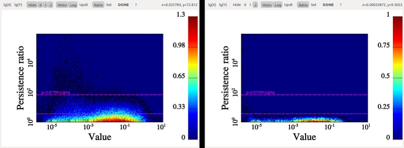
After running this command line, you should be able to visualize the following diagrams:


On this picture, the maxima/saddle persistence pairs diagram is represented on the left and the minima/saddle one on the right. The fact that the second type of pairs are clearly less persistent reflects the known fact that dark matter haloes are very prominent structures because they belong to regions in the non linear regime where density increases exponentially fast. One nice feature of persistence diagrams is that they make it easy to choose the threshold above which underlying topological structures stand out of the noise : in the present case, we want to select the high persistence tails only that clearly stand out from the bunch of pairs generated by noise. This gives us a threshold of around 3-sigmas that can be visually selected by clicking while holding Ctrl key down. Once the threshold is selected, simply press Done button.

After this operation, mse should output two files: the filaments in a skeleton type file (simu_2D.ND.NDnet_s3.up.NDskl) and the voids in a network type file (simu_2D.ND.NDnet_s3_manifolds_J0a.NDnet).

By default, mse associates maxima to vertices while minima are associated to d-simplices (where d is the dimension of space). As a result, the network representing the voids defines a set of triangles each associated to a given void. This may not be very practical for post-treatment or visualization, but we can use option -vertexAsMinima to reverse the convention (this will overwrite the previous file if the threshold is identical):

We can now visualize the result by converting the files to vtk formats using skelconv and netconv. The skeleton is smoothed and converted to vtp format:

and the input tesselation and output voids are converted to vtu format:

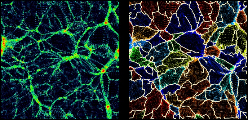
the result should look as follows when visualized with paraview: (the configuration file ${DISPERSE}/data/simu_2D_nonper.pvsm can be directly loaded in paraview (File->Load State) to produce the following plot)



Note: on the right figure, a different color is associated to the source_index of each particle depending on which void it belongs to: each void originates from a different minimum of the field and each critical point has a specific index. This source_index corresponds to the position of this critical point as a node in skeleton files or as a vertex in persistence pair networks obtained with mse (options -dumpArcs and -ppairs). It can therefore also be used to cross-link information contained in manifold networks and skeletons or persistence pairs, such as for instance retrieving the hierarchy of the voids (i.e. using the parent_index of the critical points in skeleton files and persistence pairs networks).