
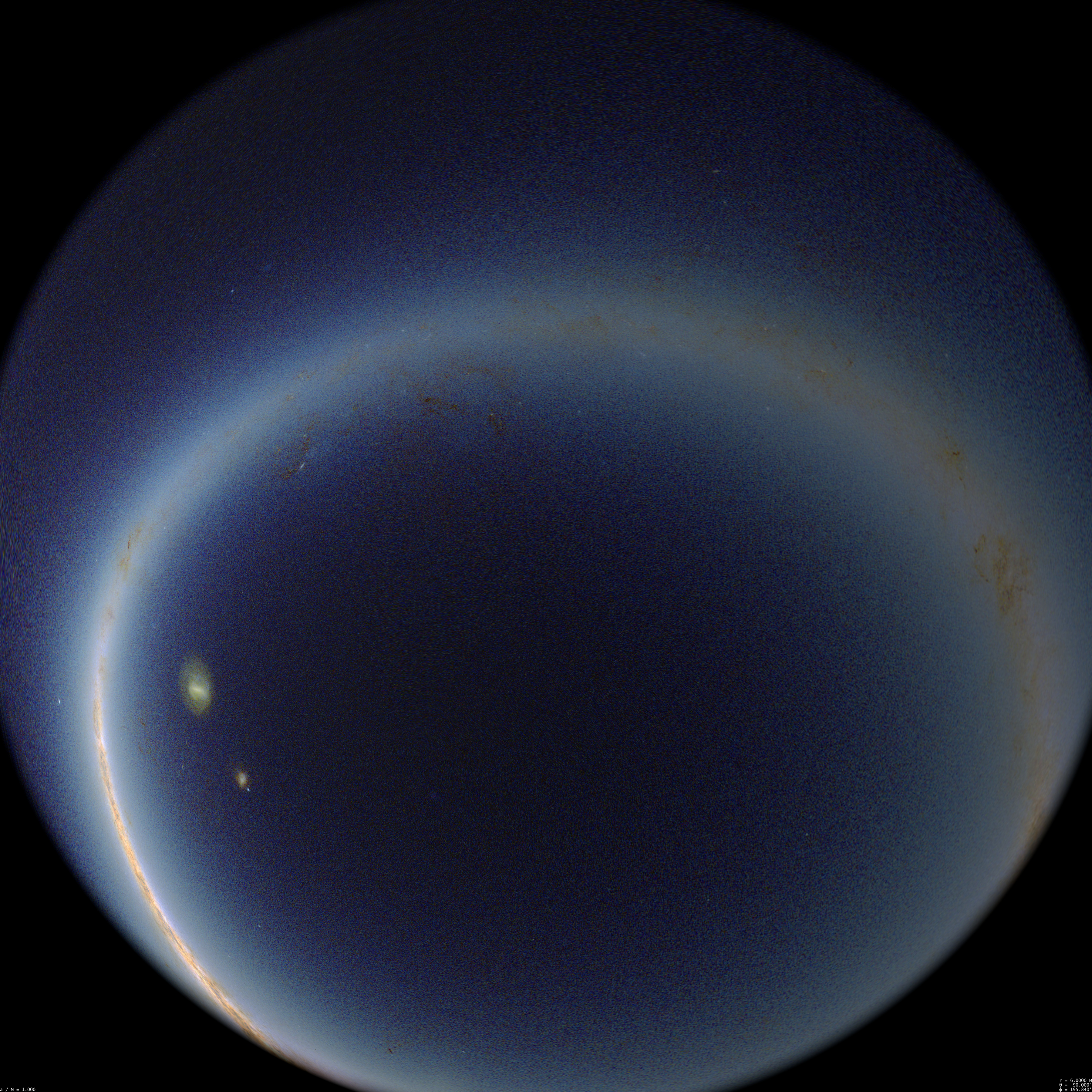
Click on the images to enlarge
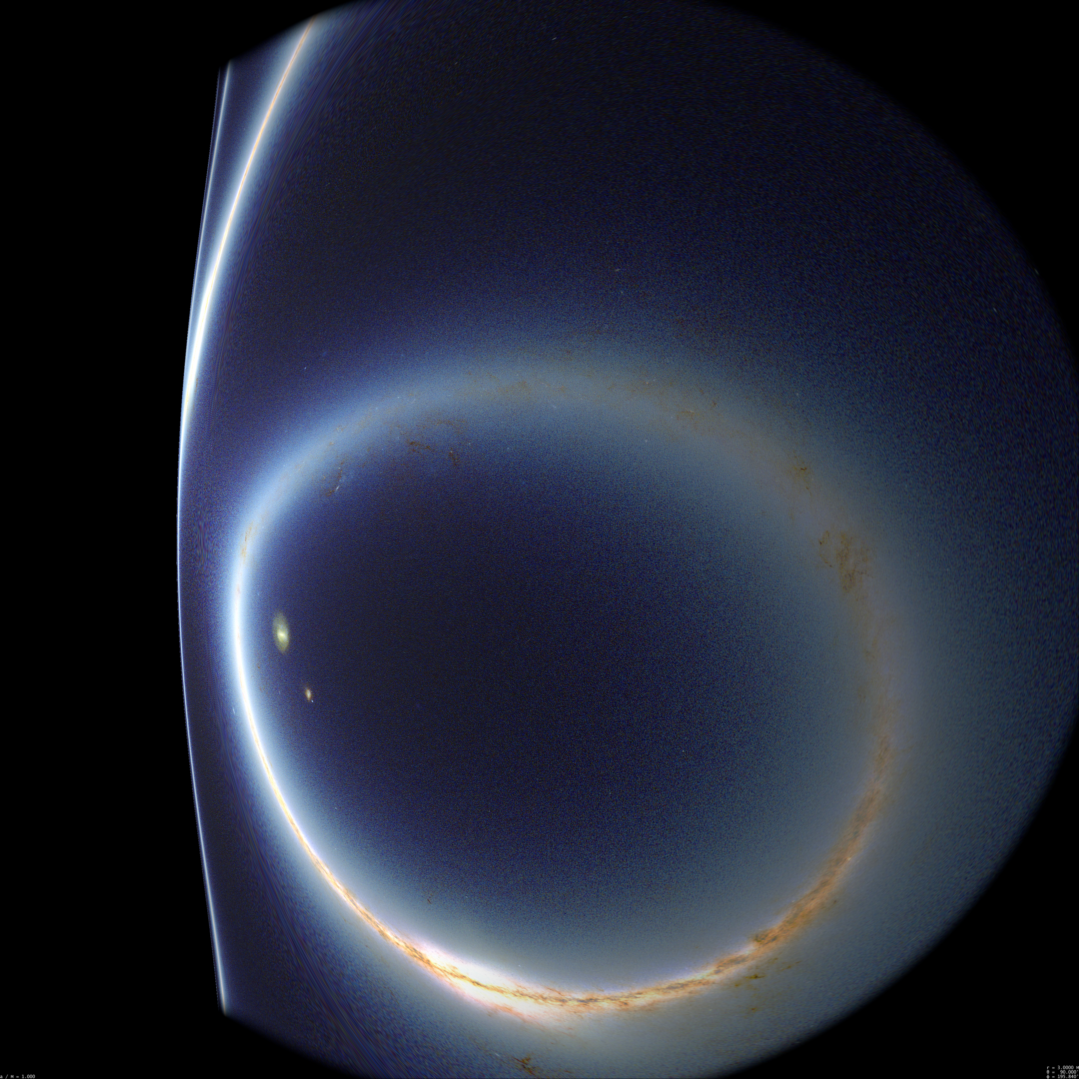
r = 3 M
This value correspond to innermost unstable null-like circular orbits in the Schwarzschild metric. However it has nothing special in the Kerr case. When getting closer to the black hole, its angular size increases, which makes it difficult to see both edges of its silhouette, even on a hemispherical image. I shall therefore compute two separate images, one showing the front direction of the observer, where he/she sees blueshifted photons along retrograde orbits, the other showing the rear direction, where the observer is caught by photons which, like him/her, travel along prograde orbits. This "prograde" (i.e., redshifted) view will be shown on the left in what follows, whereas "retrograde" (i.e., blueshifted) view will be shown on the right. Note that when r will become smaller than 2 M, i.e. when the observer is in the ergosphere, I do not really understand whether the concept of "looking in the direction where one travels" has a meaning. Nevertheless, the "front" and "rear" directions can be, at least approximatively, guessed from te variation in redshift of the direction one is looking at.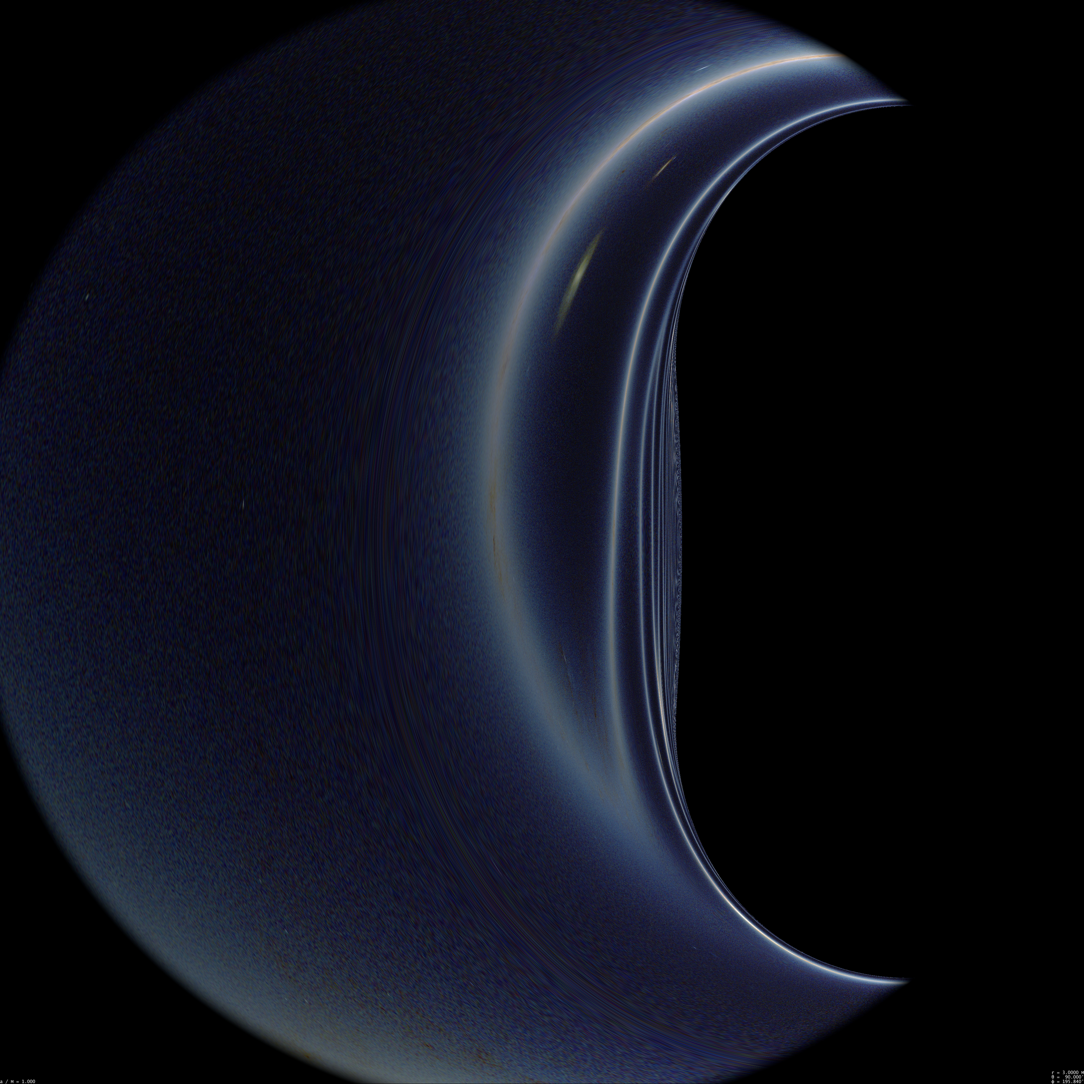
Click on the images to enlarge
r = 1.5 M


Click on the images to enlarge
Going deeper in the ergosphere
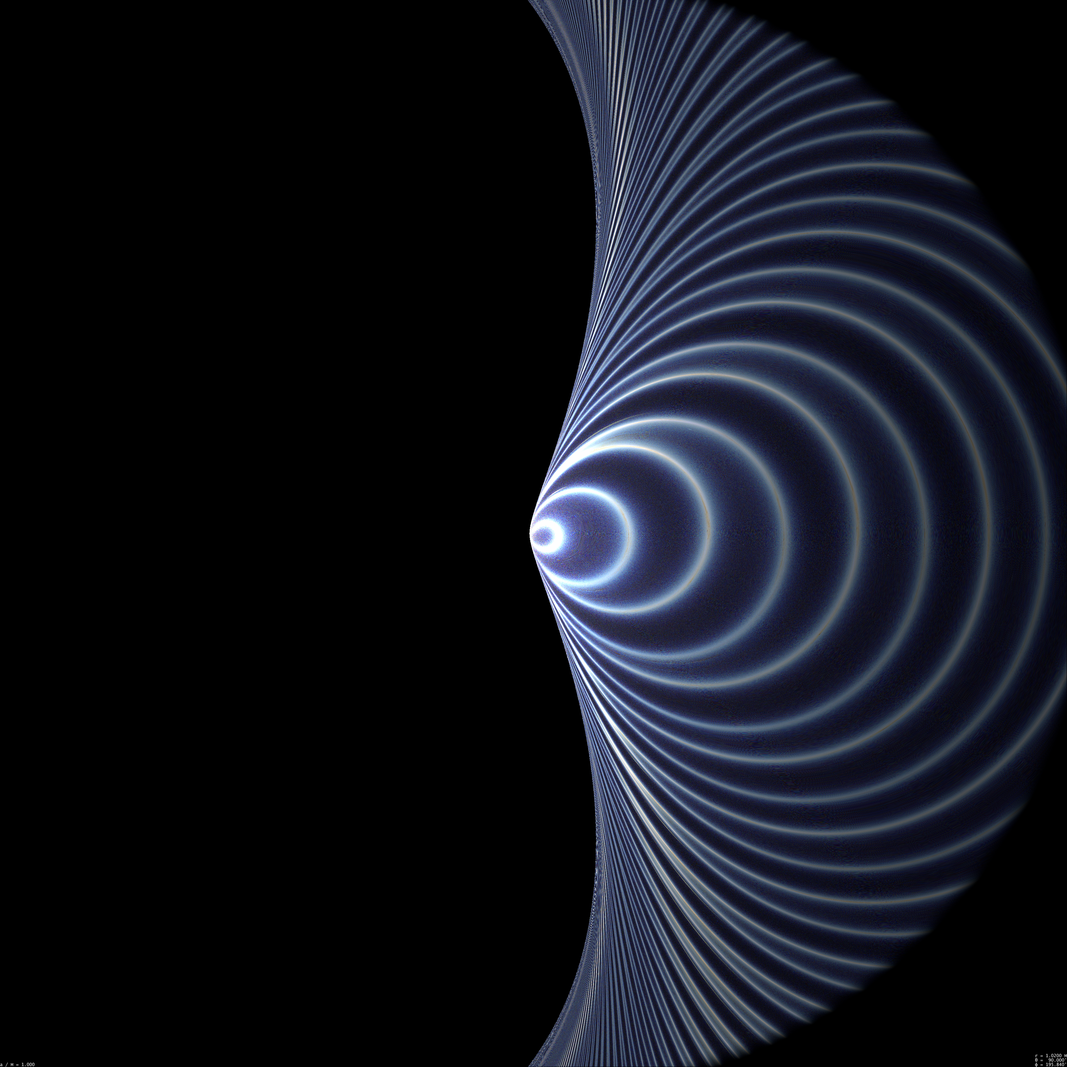
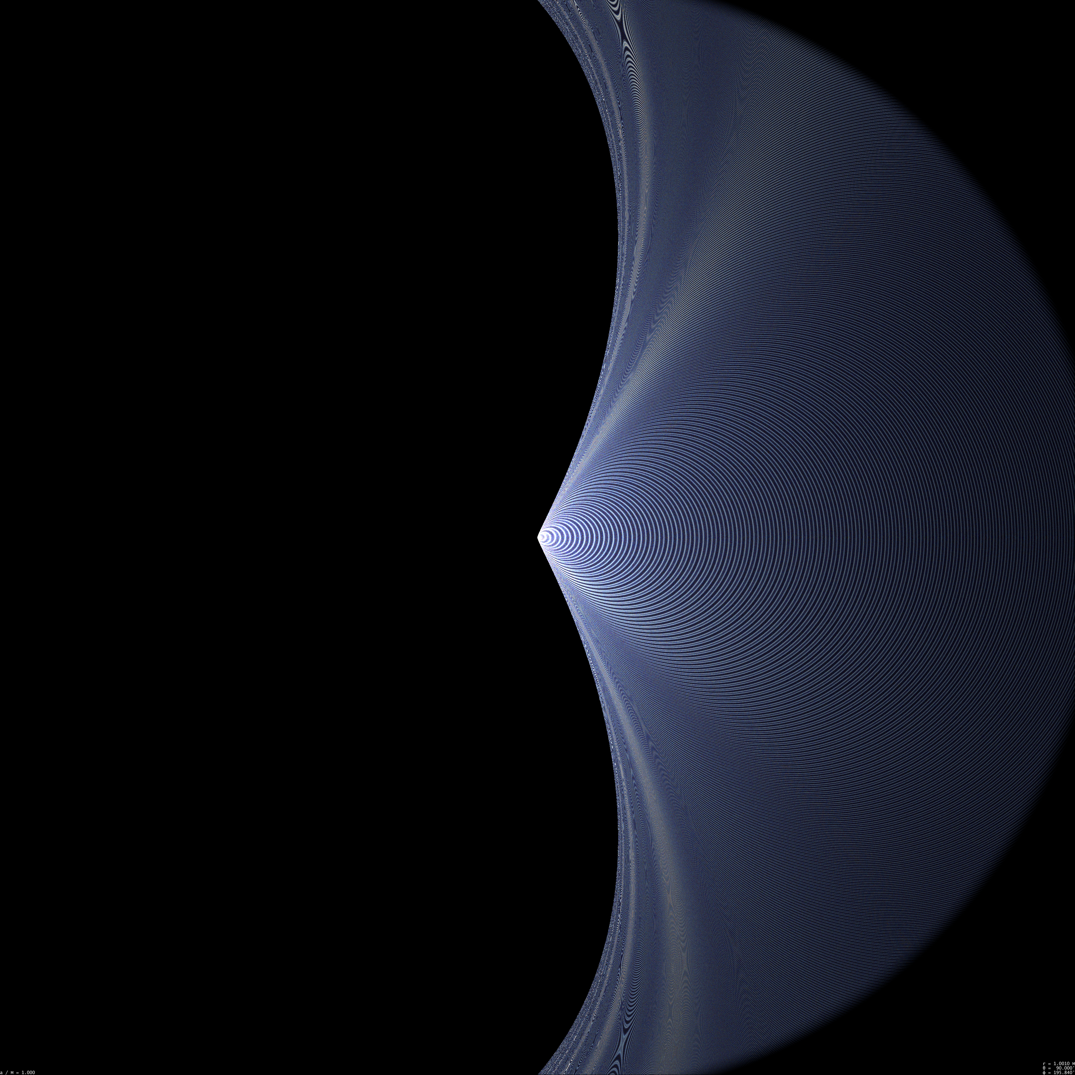
In what follows, the observer orbital radius is 1.2 M, 1.1 M, 1.05 M, 1.02 M, 1.01 M, 1.005 M, 1.002 M, 1.001 M, 1.0005 M, 1.0002 M and 1.0001 M, respectively. The thickness of the celestial sphere ghost images increases as r decreases. the view at r =1.01 M is quite aesthetic. On the prograde view, some bubble-like structures are easier and easier to spot as r decreases. These are definitely unphysical moiré-like pattern due to an insufficient resolution of the images. When seen at higher resolution, these structures disappear, but actually reappear closer to the black hole silhouette since they are also due to the fact that the image resolution is again insufficient as one looks closer and closer to the edge of the black hole. Note that for small r (1.005 M, say) you need to click on the picture to enlarge it in order to see the full scope of multiple images. However, even at full 3600×3600 resolution, the smaller r image not longer manages to see all of them. Visualizing the full richness of the image necessitates an increasing resolution as r decreases!

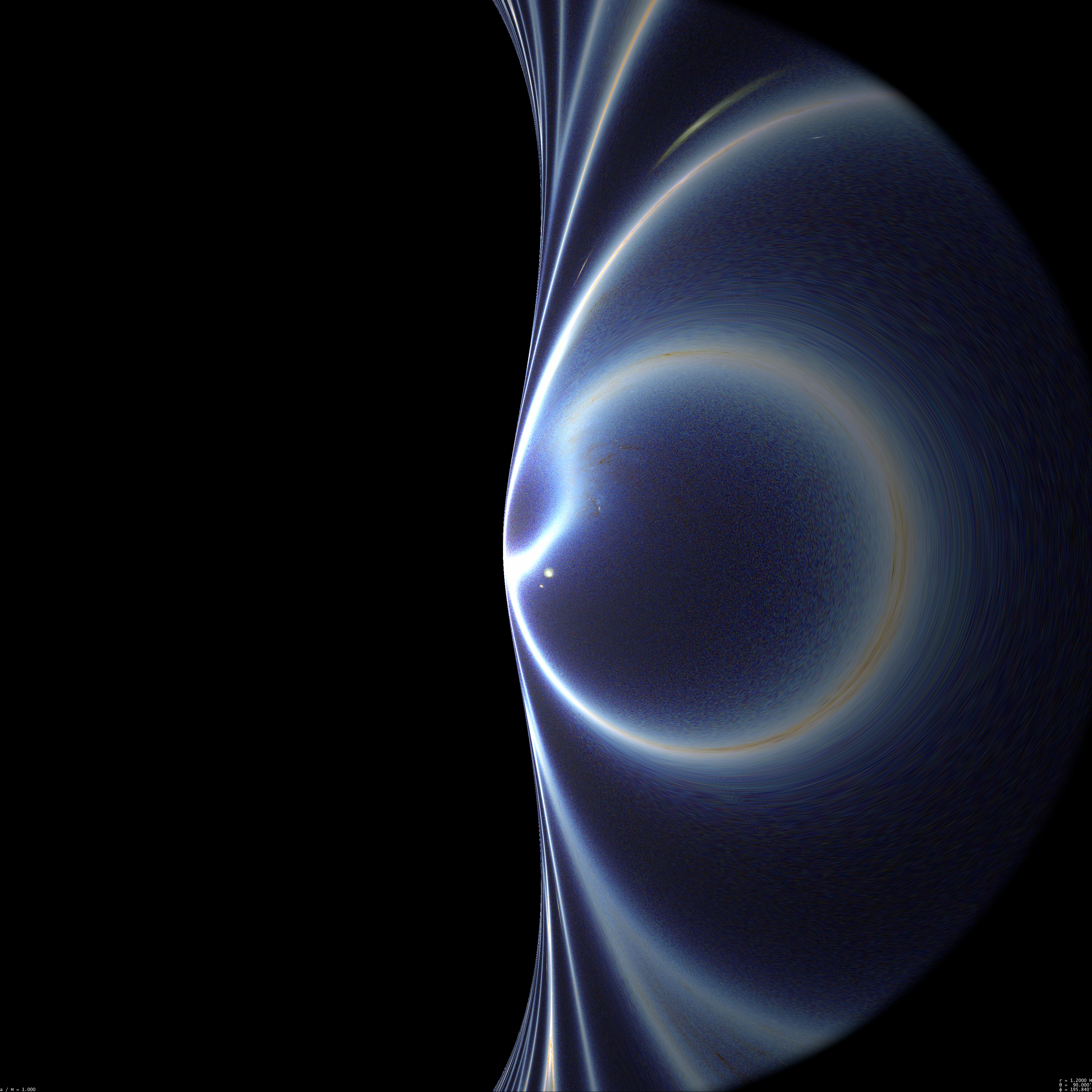
r = 1.2 M; Click on the images to enlarge

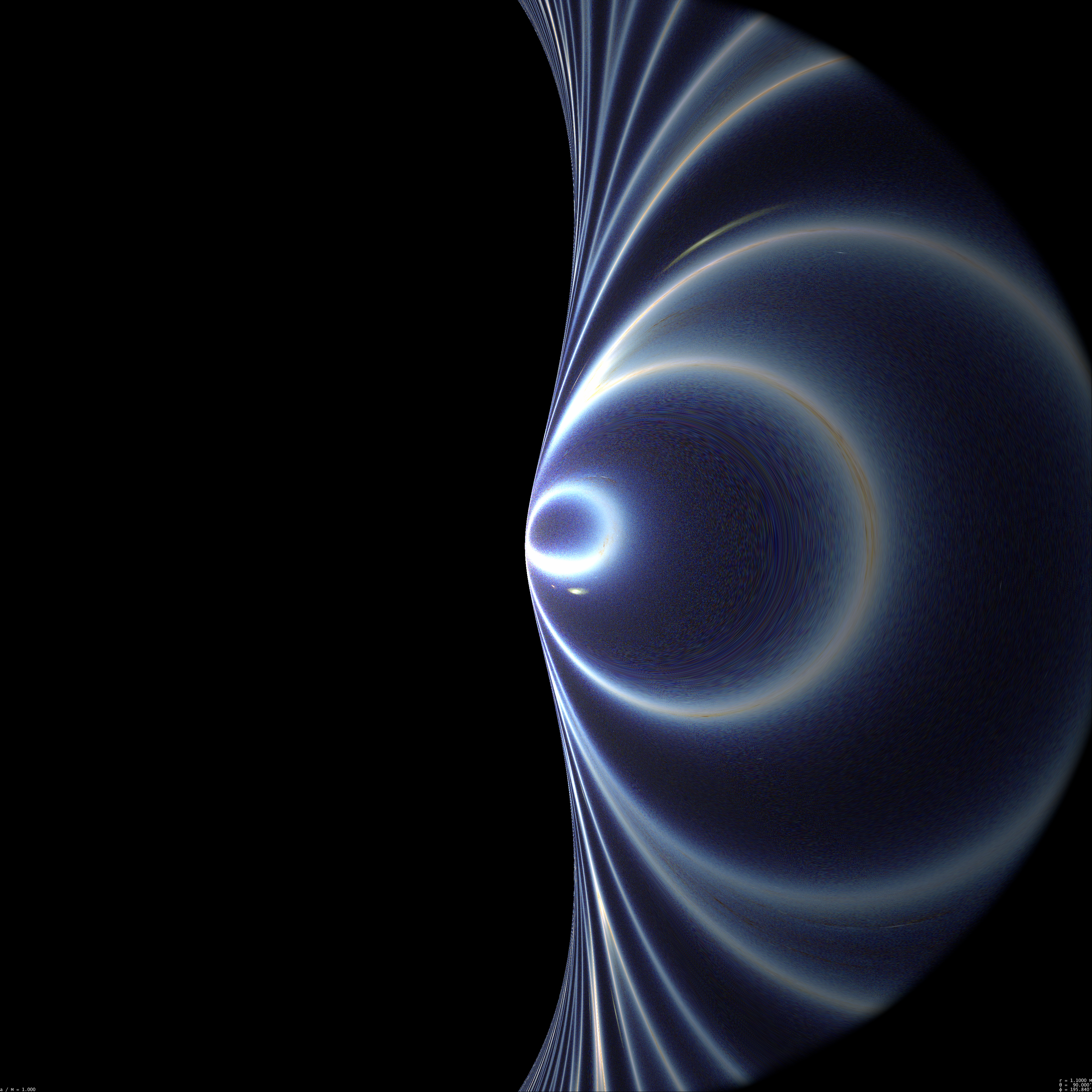
r = 1.1 M; Click on the images to enlarge
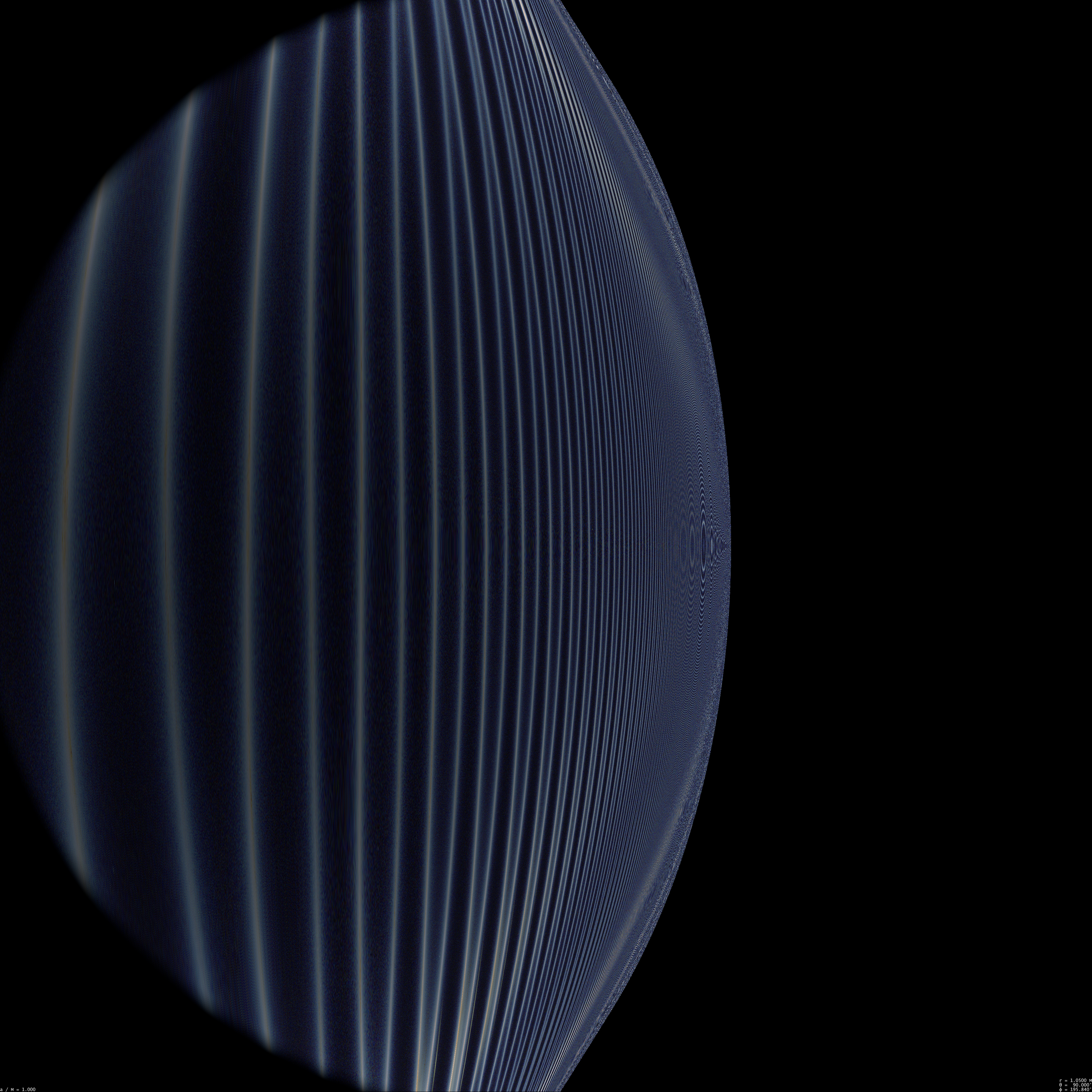
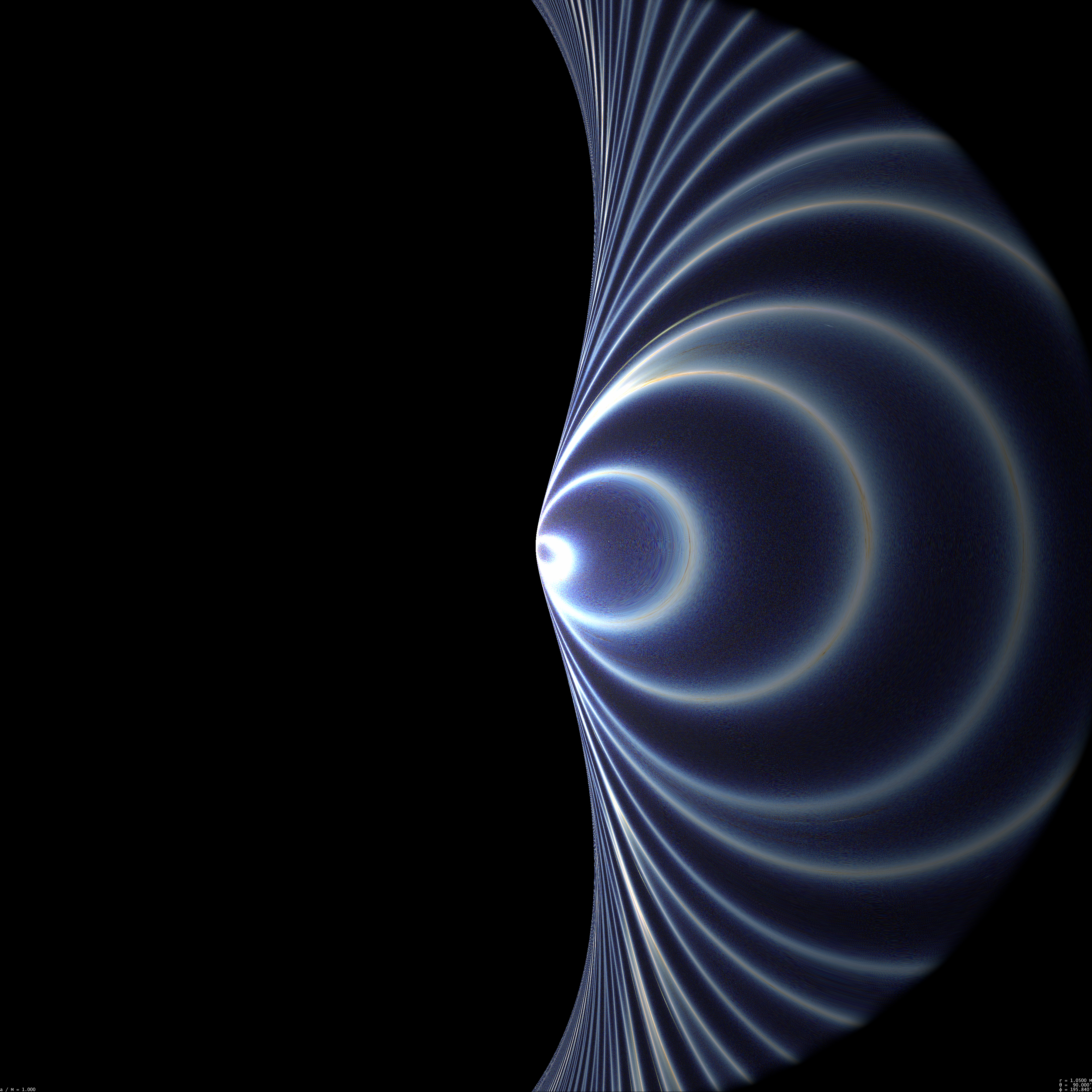
r = 1.05 M; Click on the images to enlarge
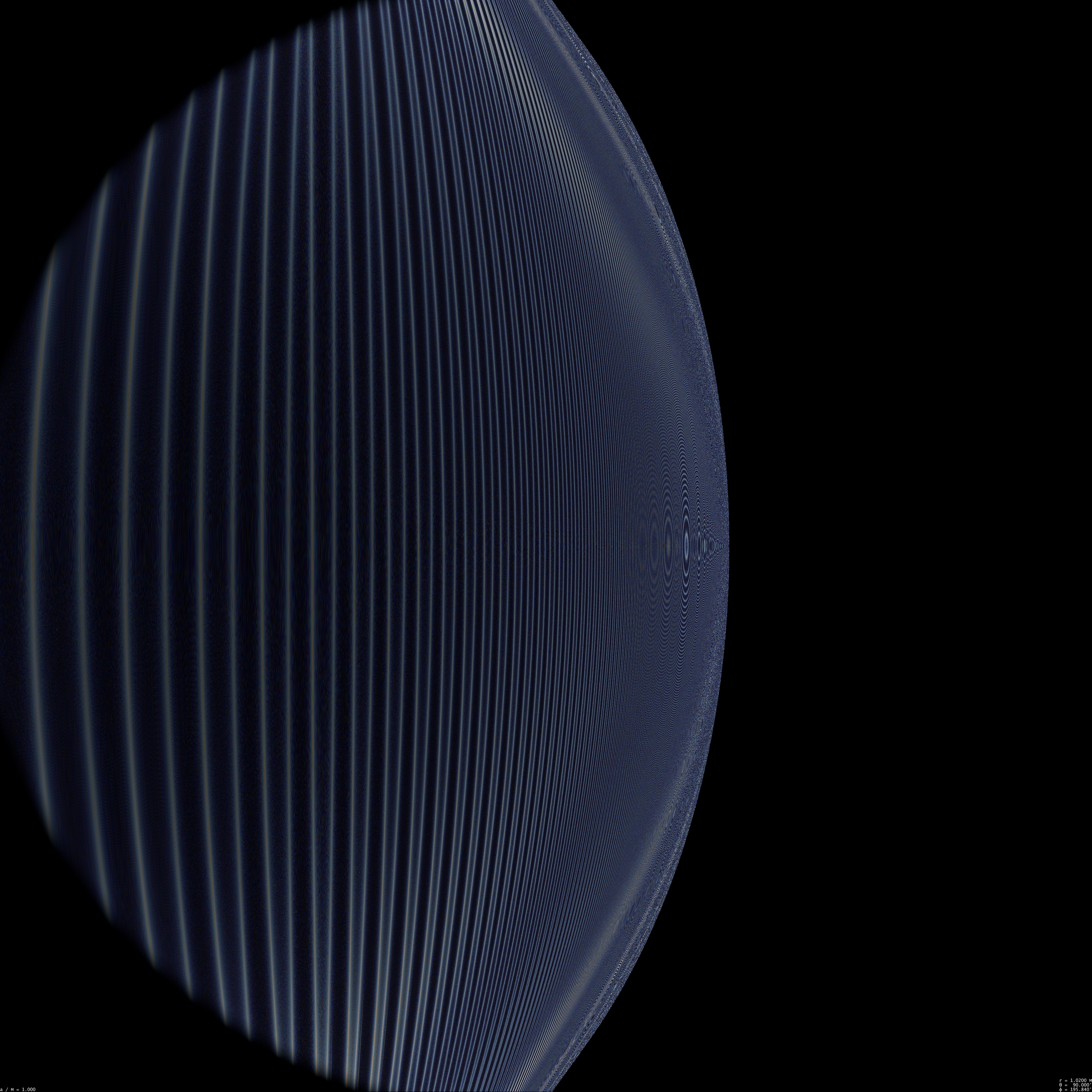
r = 1.02 M; Click on the images to enlarge
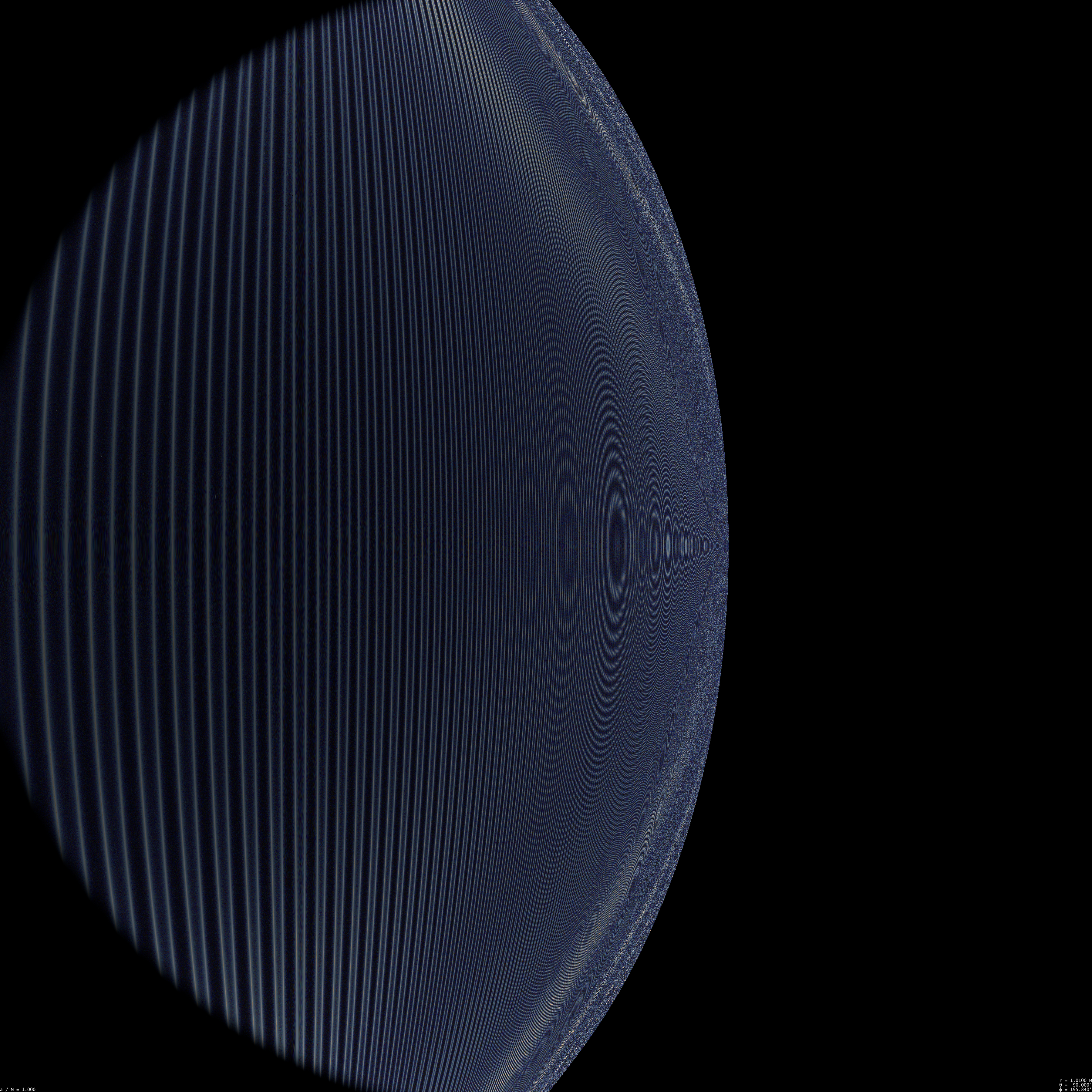
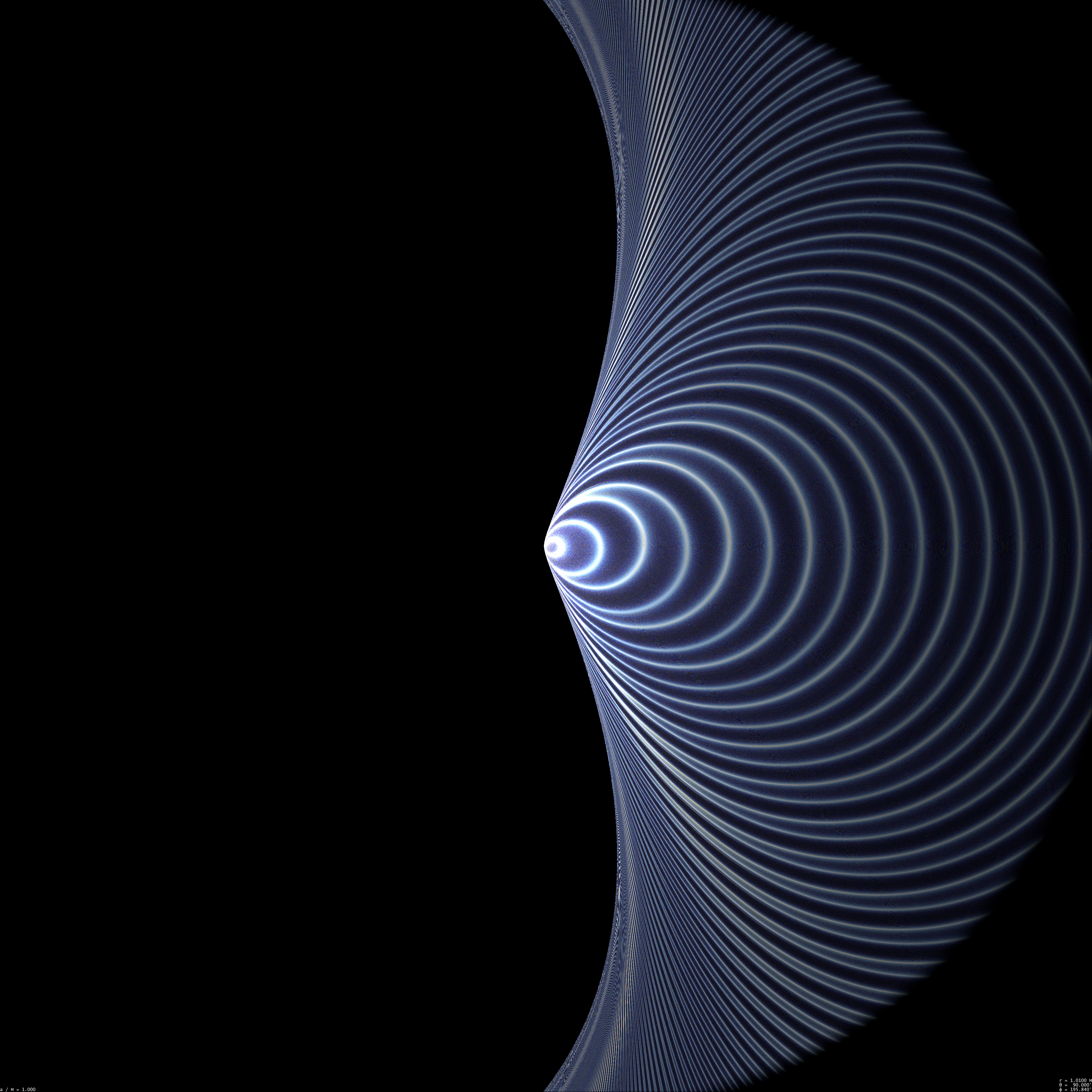
r = 1.01 M; Click on the images to enlarge
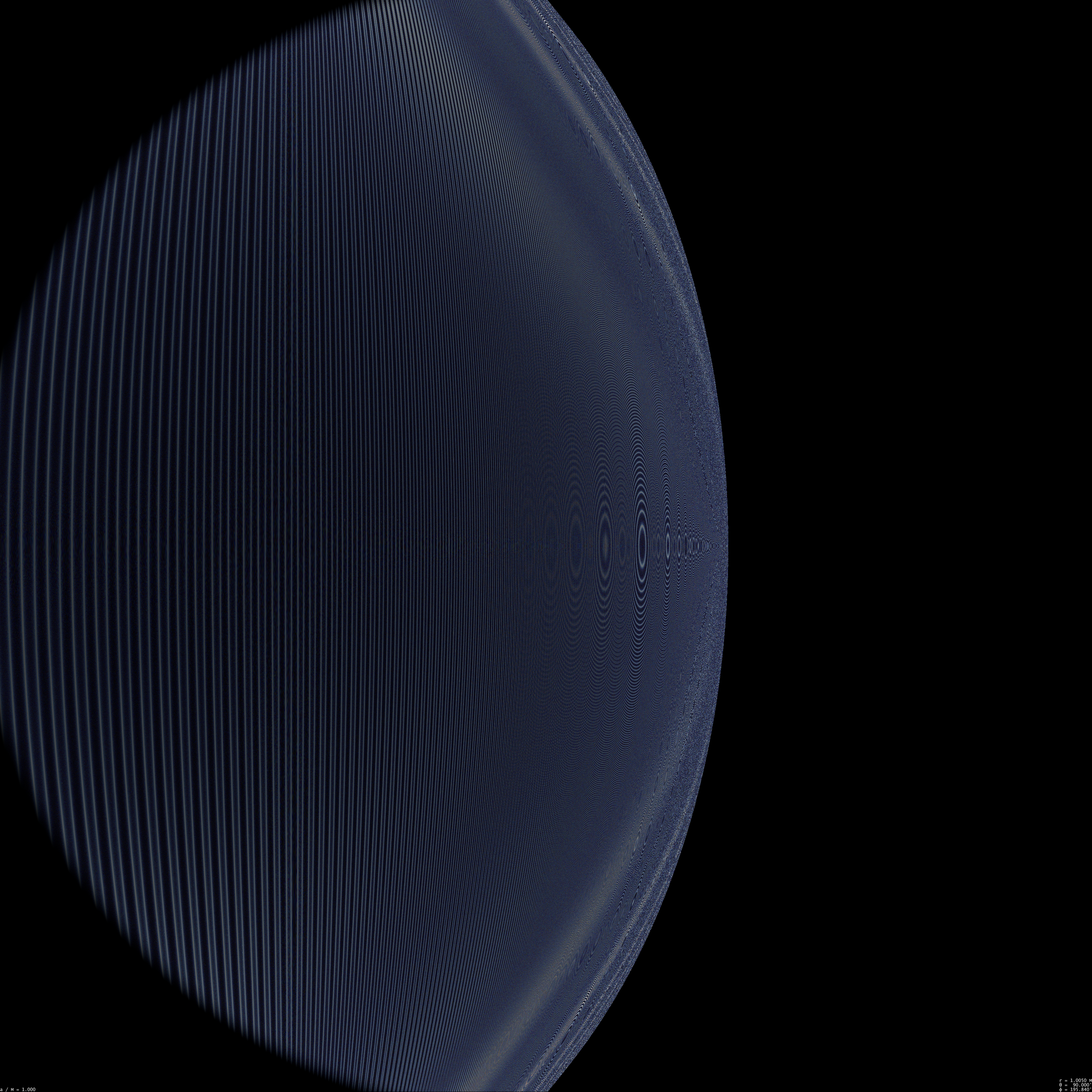
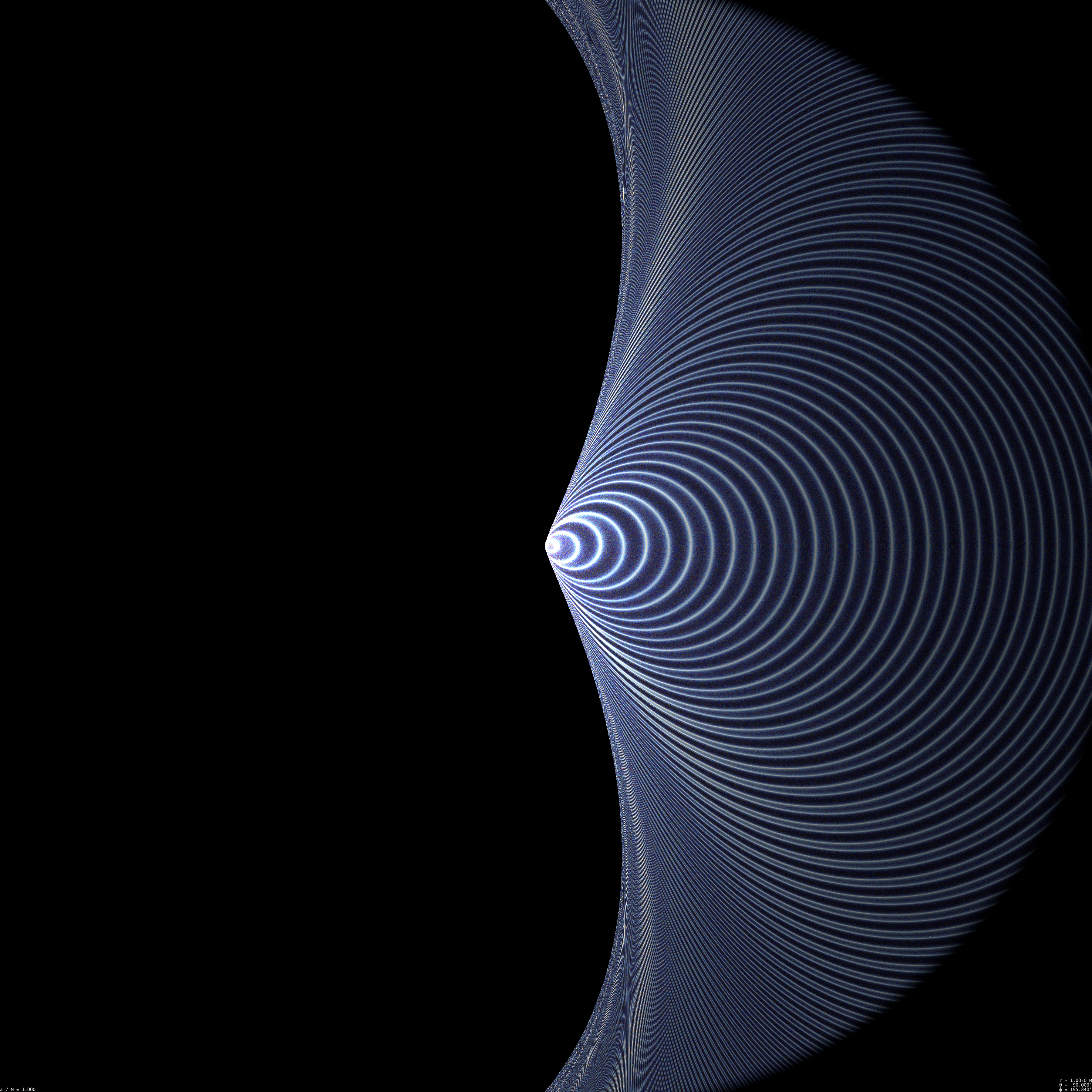
r = 1.005 M; Click on the images to enlarge
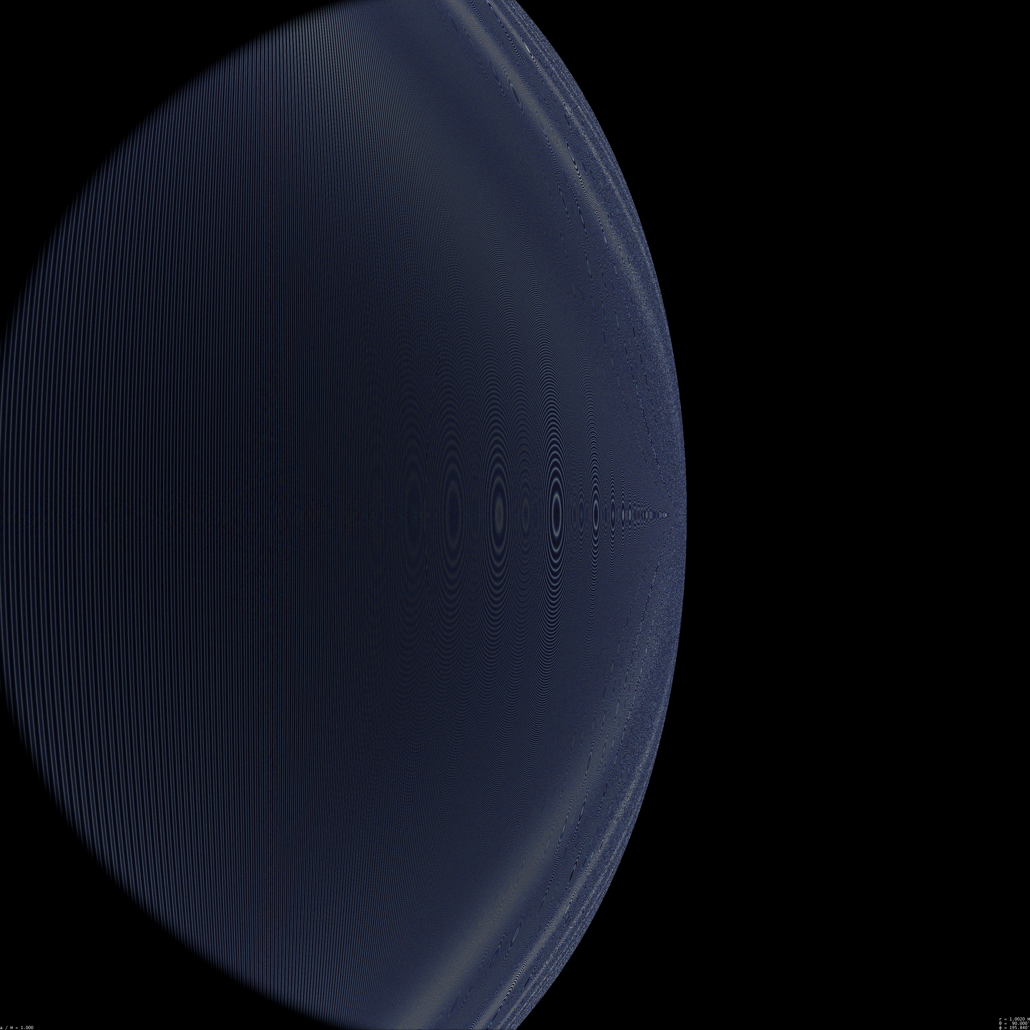
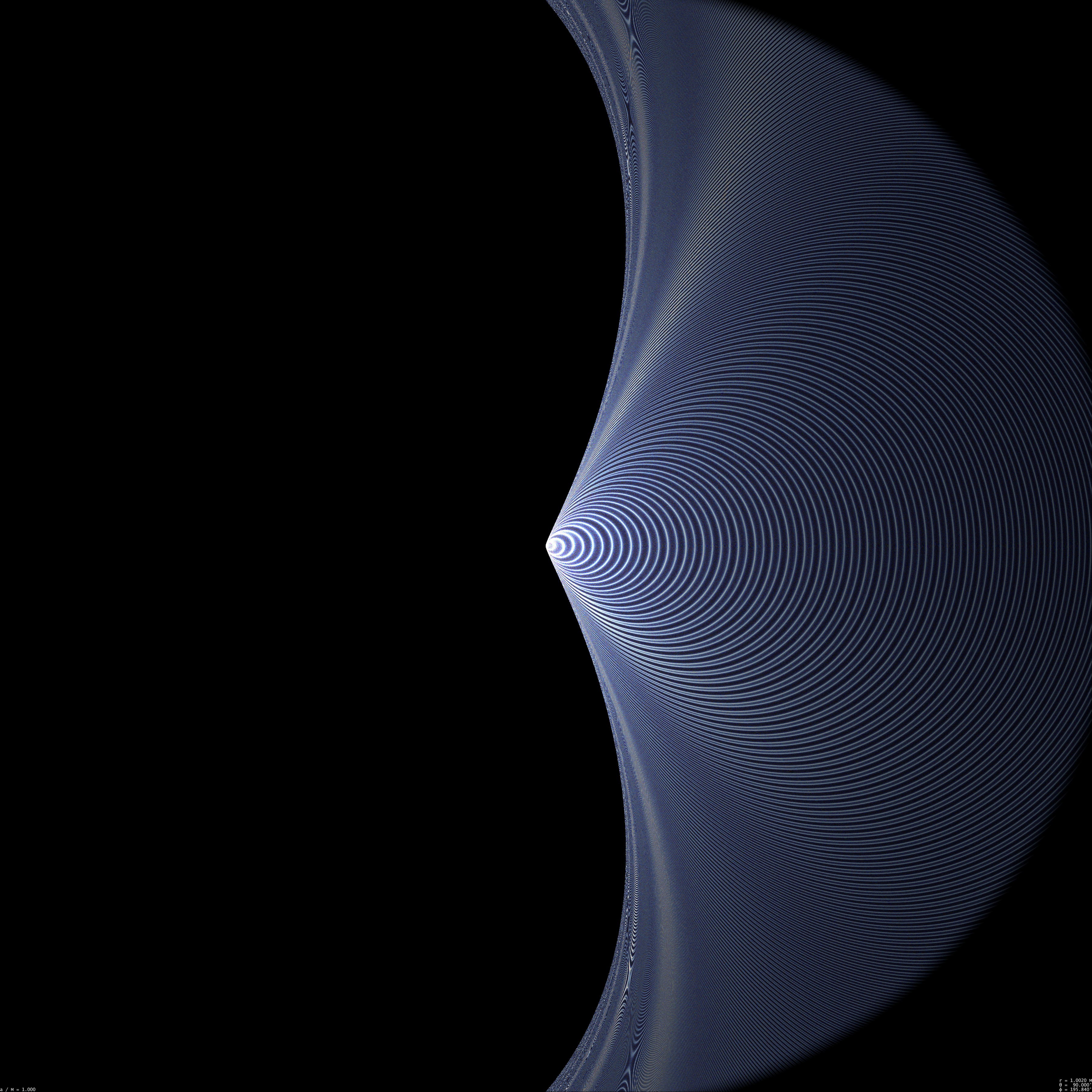
r = 1.002 M; Click on the images to enlarge
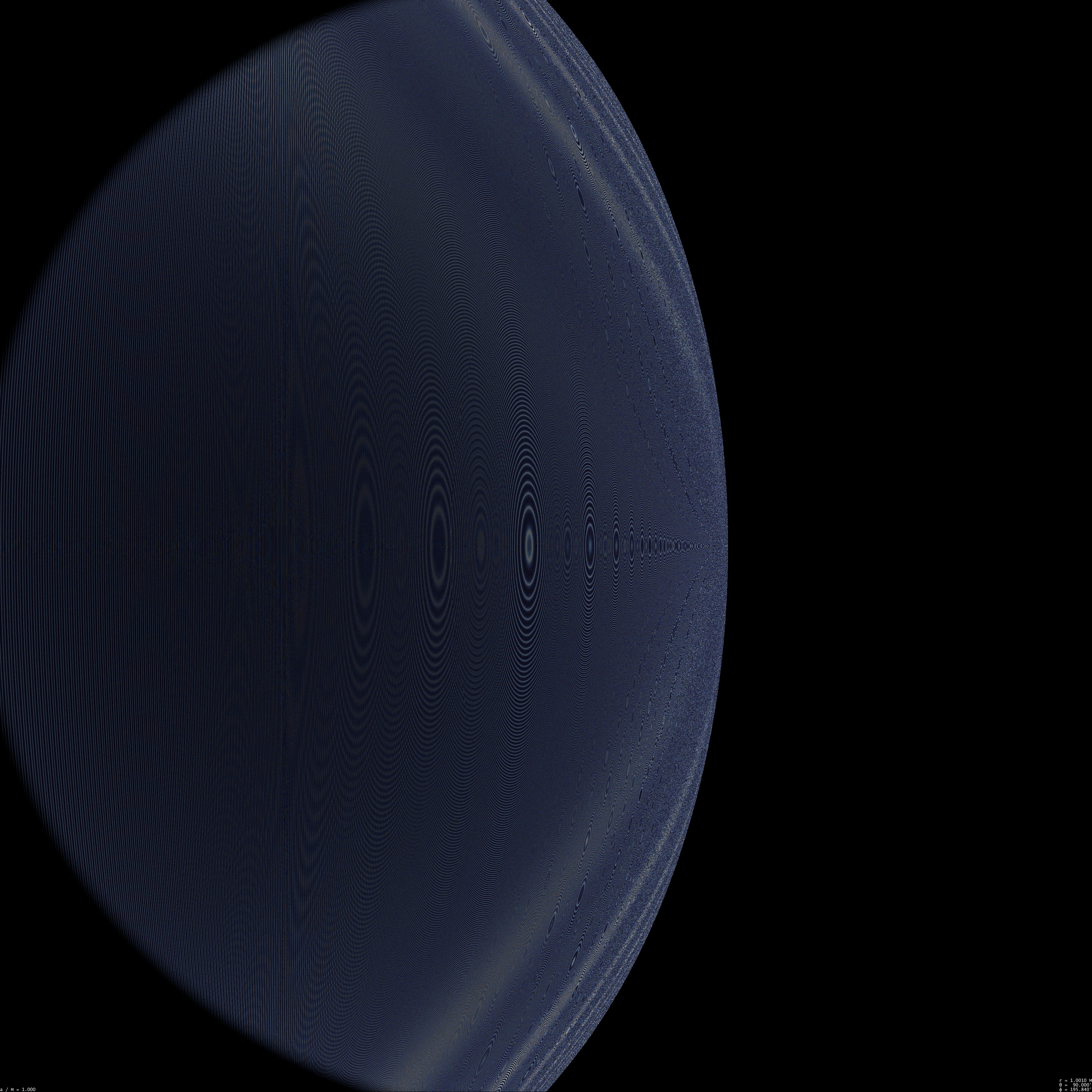
r = 1.001 M; Click on the images to enlarge
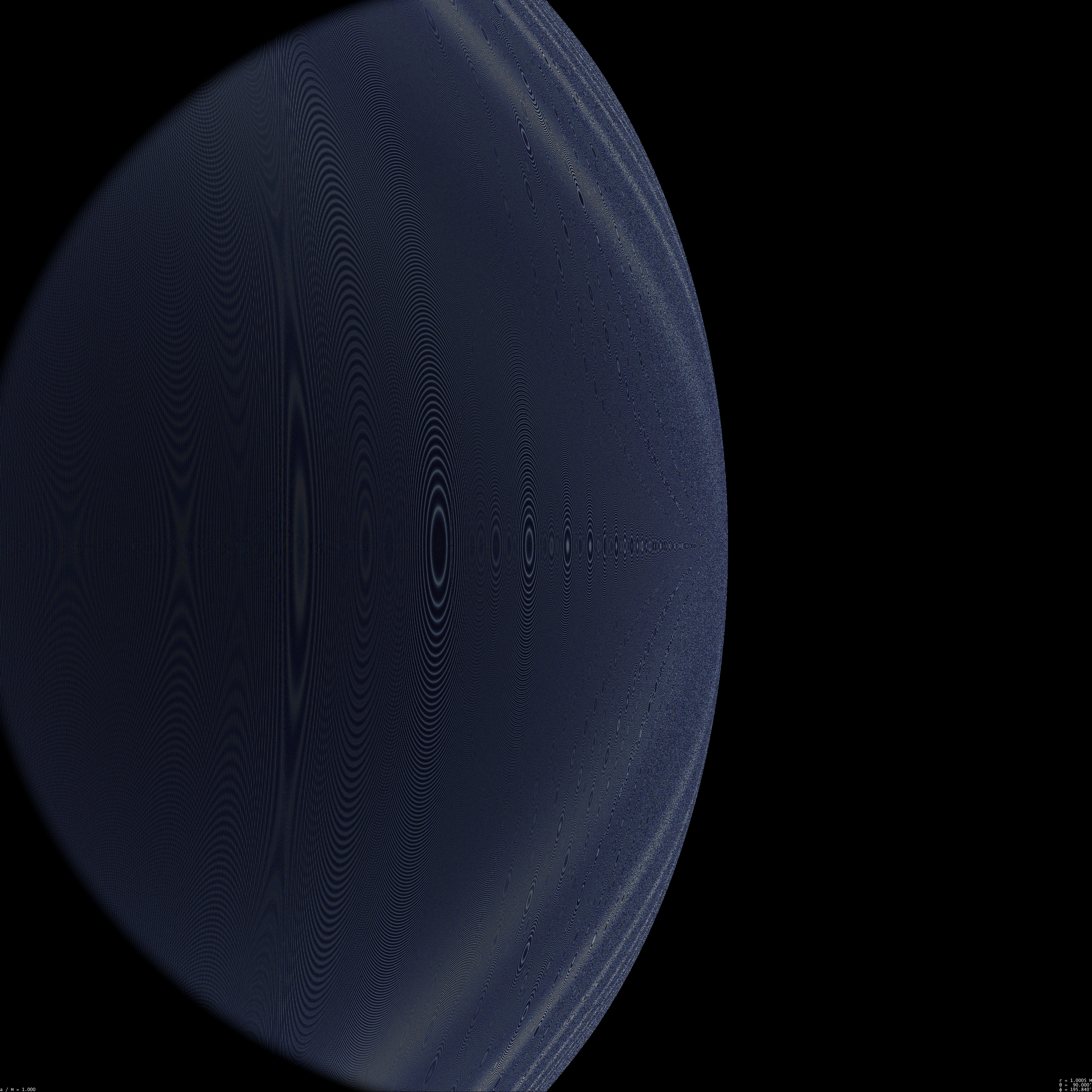
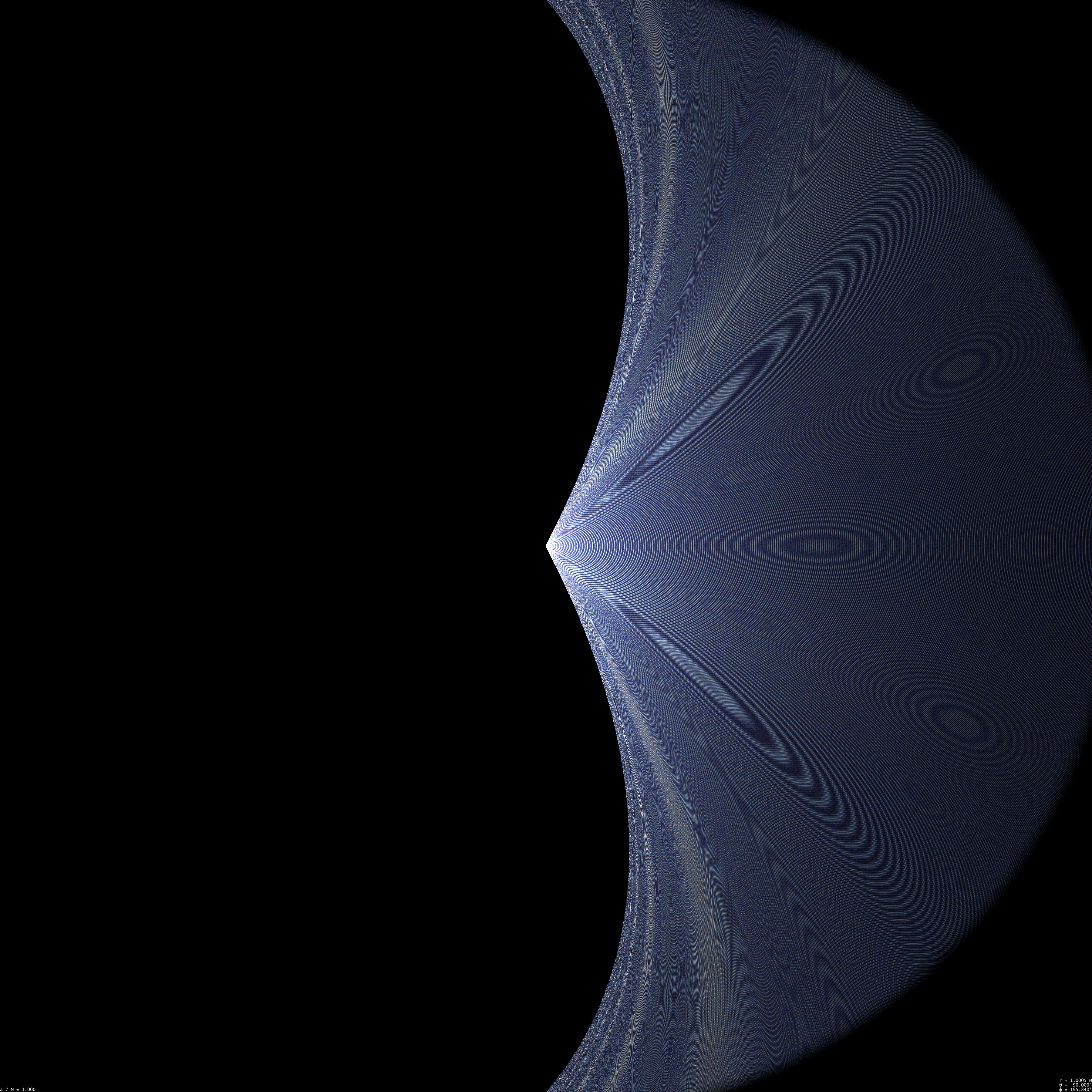
r = 1.0005 M; Click on the images to enlarge
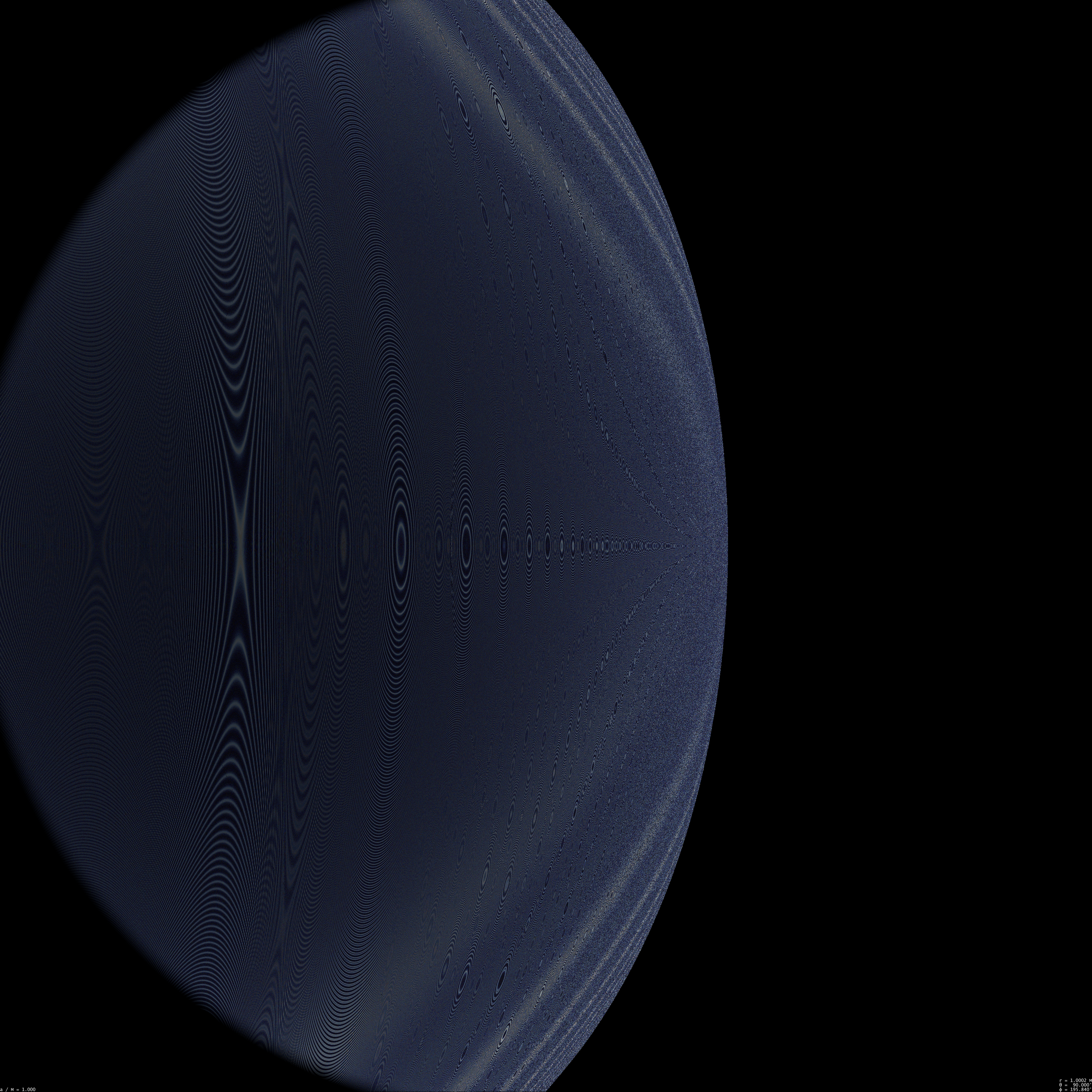

r = 1.0002 M; Click on the images to enlarge
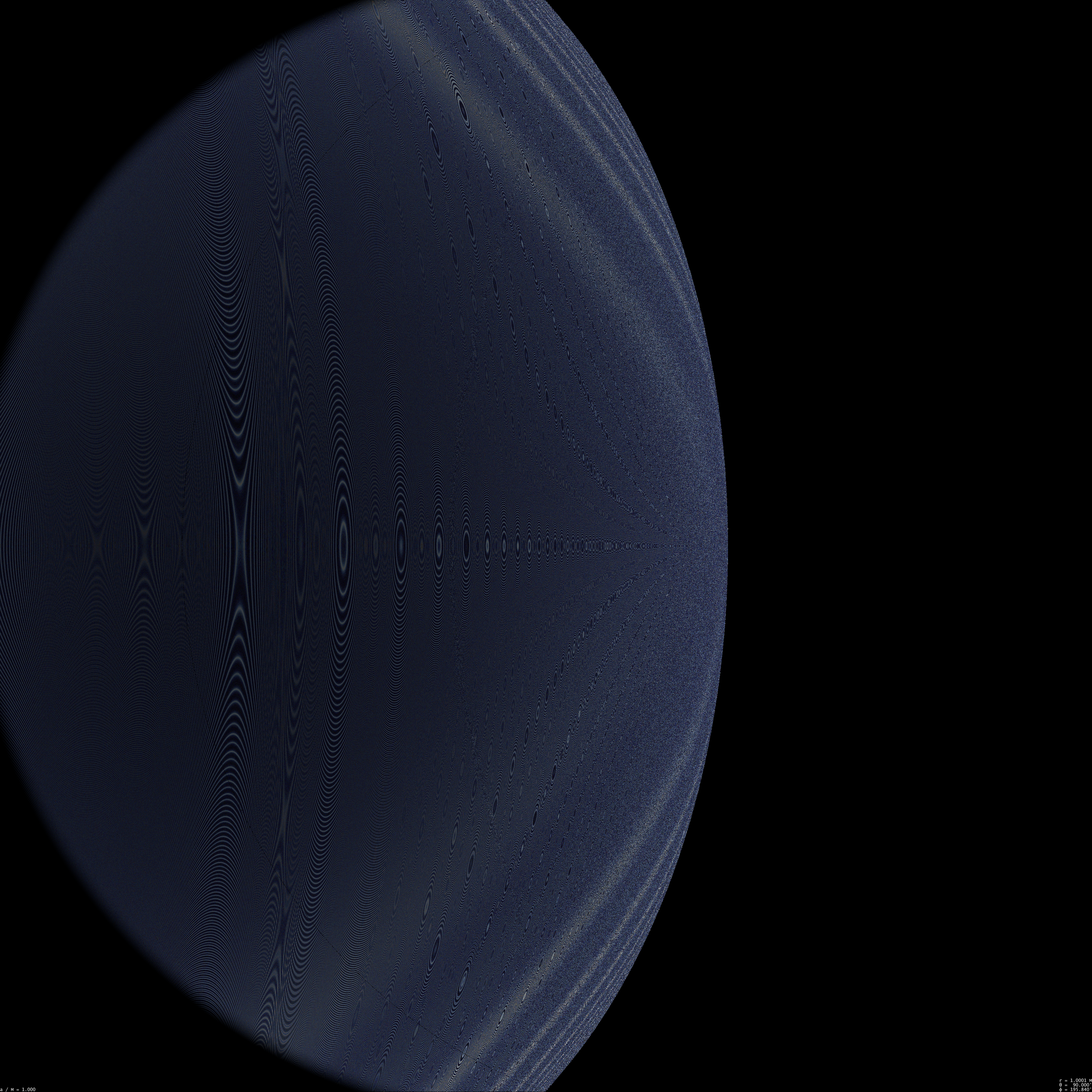

r = 1.0001 M; Click on the images to enlarge
What happens below r = 1.0001 M?
At the moment of writing, my code experiences a series of problems for r < 1.0001 M in addition to becoming extremely slow. I presume that the number of ghost images of significant angular size will be ever increasing as the orbit gets closer and closer to the black hole, however, I have not yet been able to check this.Videos
For the 7 first values of r shown above, the images above are actually the first frame of 1800 frame long videos which all show a complete orbit around the black hole. Therefore, each video runs in 1 minute or 1'12", depending whether your player runs at 30 or 25 frames per second. Of course, the actual orbital period has to be scaled with the corresponding value of M one uses. An important thing to note is that when close to the black hole, the angular distance between the primary image of the Milky Way and its first ghost images is rather small (less than 10 degrees, say, for r = 1.02 M, and far less for smaller r). This means that when the observer makes one turn around the black hole, then the whole celestial sphere is moving on the right by only 10 degrees, each image of it replacing the next one! In other words, for a fixed orbital period, the angular displacement of the celestial sphere is much larger for large orbital radius than for a small one. Whether or not this is compensated by the fact that the orbital period at fixed M decreases with r is not known to me at the time of writing, however, it might happen that, contrarily to naive expectation, the view seen by an orbiting observer becomes almost still as r approaches the horizon!
| r
/ M |
Progade
view |
Retrograde
view |
| 6 |
circ_6_000c_dm2q.mpg |
circ_6_000c_dm1q.mpg |
| 3 |
circ_3_000c_dm2q.mpg |
circ_3_000c_dm1q.mpg |
| 1.5 |
circ_1_500c_dm2q.mpg |
circ_1_500c_dm1q.mpg |
| 1.2 |
circ_1_200c_dm2q.mpg |
circ_1_200c_dm1q.mpg |
| 1.1 |
circ_1_100c_dm2q.mpg |
circ_1_100c_dm1q.mpg |
| 1.05 |
circ_1_050c_dm2q.mpg |
circ_1_050c_dm1q.mpg |
| 1.02 |
circ_1_020c_dm2q.mpg |
circ_1_020c_dm1q.mpg |